This slide presentation describes the basics of the age reliability relationship. It clarifies the difference between the Failure Rate function and the Conditional Probability of Failure.
An amusing story about confusing Failure Rate and Conditional Failure Probability is told in this post.
John Moubray, as a warning against being too sure of oneself, used to tell this story to his aspiring RCM consultants:
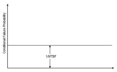
A newly trained RCM practitioner consultant was delivering the standard three-day RCM course to a group of his clients, when the subject of random failure came up. The consultant drew the following graph on the white board.
Random Failure Conditional Probability Of Failure Graph
One of the students commented that this graph was wrong. The dissenting student stated that the conditional probability of failure was not exactly equal to the inverse of the mean time between failure. The consultant stood his ground. A heated argument broke out almost ending in fisticuffs. Bitterness permeated the remainder of the course.
Moubray said that the student was right and the consultant was wrong. He went on to add that the graph ceases to be true if the MTTF is less than four arbitrary time units.
What is the explanation for this? Isn’t the conditional probability of failure exactly equal to the inverse of the MTBF for a randomly failing item? The consultant fell victim to the common confusion of the Failure Rate function (also called “Hazard rate” or “Hazard function”) with Conditional Probability of failure. RCM practitioners and maintenance engineers tend to think in terms of the latter, while mathematicians and statisticians use the former in their theoretical work. The consultant could have remained on safe ground had he labeled the vertical axis “h(t)” or “hazard” or “failure rate”. Here is the explanation for Moubray’s statement.
The left hand side of the following equation is the definition of the conditional probability of failure.
Don’t be intimidated by the mathematical symbols in Eqn. 1. The equation simply states in mathematical terms that the conditional probability of failure in any interval Δt is equal to the probability of a brand new item failing before time Δt. This would be the case for random failure.
Also for random failure, we know (by definition) that the (cumulative) probability of failure at some time prior to Δt is given by:
Now let MTTF = kΔt and let Δt = 1 arbitrary time unit. Then the Conditional Probability of failure is
exactly.
Now let’s write ex as its infinite series
Then for x = -1/k
Rearranging, the Conditional Probability is
exactly, or
approximately.
Let’s calculate the exact and approximate values (by using the first term and the first two terms of the infinite series expansion for ex) for the conditional probability of failure in the table:
MTBF/time unit
Exact
Approx.
k=2
0.3935
0.5
k=3
0.2835
0.333
k=4
0.2212
0.25
k=5
0.1813
0.2
k=6
0.1535
0.1667
k=7
0.1331
0.1429
k=8
0.1125
0.125
Knowing that k=MTBF/Δt, we can see that if the MTBF is large relative to the age unit Δt, the conditional probability of failure is well approximated by the inverse of the MTBF. From the table, Moubray’s factor of 4 is not bad (since 0.22≈.25).
A more detailed explanation of the difference between Conditional Failure Probability and Failure rate can be found in the post “Time to Failure“[2].
[1]This relationship reads as follows: “The probability that the item will fail in an interval between t and t+Δt (given that X ≥ t) is equal to its failure probability between 0 and Δt” which would be true for random failure behavior.↩
[…] Note that the Reliability as calculated by the equation for random failure is slightly different from that calculated in the previous worksheet. That is because the equation represents a continuous function while the Survivors were calculated at discreet intervals. For more on discrete versus continuous functions, see the article here. […]


 exactly, or
 approximately.

Leave a Reply
You must be logged in to post a comment.