EXAKT basic tutorial

This tutorial can be run using the EXAKT program. Please download  a fully functional trial version. Tutorial 1 will familiarize you with the basics of Weibull PHM analysis, how to create an optimal CBM model, and how to deploy it through an agent. The instructions in black are minimal so as to keep them simple. The purple colored text provides more detailed explanation.

Whenever an EXAKT menu item is mentioned in bold, it should be left-clicked in the EXAKT program. When other items are mentioned, usually, they should be double clicked. X indicates that you should close the active sub-window.

When you expand a sub-window and then close it, you will lose the familiar arrangement of underlying windows. When this happens, simply reduce the underlying window or hit the Mov Win Left icon.These general rules will not be repeated. You may either print out this tutorial or you may resize and position this document or mindmap elsewhere on your screen. Similarly, you may resize and position the EXAKT program. When necessary, you can temporarily expand the EXAKT window to full screen.

What will you learn in this tutorial?

You will learn the basic functions of the EXAKT model building software and the EXAKT decision agent software. You will use a reduced set of oil analysis data from a fleet of haul truck transmissions to build a proportional hazards model. Then you will deploy this model as an “intelligent agent” that silently and automatically monitors future condition monitoring data, returning an optimized decision (whether or not to remove and repair the transmission) as each new set of condition monitoring readings are received.

A long term policy of making optimized decisions will, on the average, minimize some undesirable feature, such as cost , or maximize some wanted feature, such as availability. The agent provides a remaining useful life estimate based on the current condition of the equipment, its age, and all relevant maintenance and operational events that have occurred.

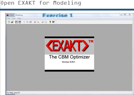
Launch EXAKT

Start, Exakt for Modelling

Download the data file. Extract the database files (Transmission_MES.mdb and Transmission_DMDR.mdb) in a folder, say in “\ExaktBasic” on your hard drive.

Launch “EXAKT for Modelling”. This is the program for validating and analyzing condition monitoring and event data and for building the optimized CBM (condition based maintenance) model.

Create a database (document) for the model

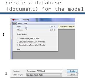
File, New, Navigate to the folder where you placed the Transmission_MES.mdb file, File name: Transmission_WMOD.mdb, Create

A “model” refers to a failure mode, in context as defined in the RCM knowledge base. Specifically a CBM model describes a failure mode’s behavior in terms of its age and significant monitored variables.

A decision model, we’ll see later, incorporates business factors in order to optimize the CBM decision with respect to an optimizing objective, for example, maximum availability.

Connect the model to the age and CBM data

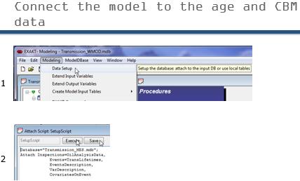
Modeling (on menu bar), Data Setup, Enter the following into the script editor:

 

 

 

 

 

Database="Transmission_MES.mdb";
 Attach Inspections=OilAnalysisData,
 Events=TransLifetimes,
 EventsDescription,
 VarDescription,
 CovariatesOnEvent

Execute, Save

Examine the above attachment script. You will note that it creates an ODBC (open database connectivity) link to an external database called “Transmission_MES.mdb.” Then it has “attached” a number of tables. It has applied its own internal names to two of the tables using the A=B syntax but other tables are attached directly since their names are already consistent with EXAKT’s internal names for those tables.

Notice that the attached tables have now become visible and accessible in the tree view in the left window pane. In the next steps you will examine each one of those tables to become familiar with their content and structure.

Examine the Inspections table

Inspections

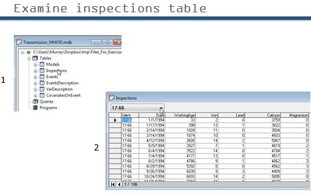
Open the Inspections table by double clicking on it. Note the column names and content. Ident, Date, and WorkingAge are key words used by EXAKT. “Ident” is the unique name of each unit of a specific type of Item to be analyzed.

An item is a significant system, subsystem,  component, part, or failure mode upon which it is convenient and desirable to conduct reliability analysis. An item may consist of several components and may be subject to several failure modes. In this introductory tutorial we’ll keep it simple and assume that the item is a simple item with a single failure mode, namely “Transmission fails”.

The “Date” may be set up in date or in date/time format. If condition monitoring inspections are more frequent than once every 24 hours, the date/time format must be used. The WorkingAge is a measure such as hours of operation, fuel consumed, thousands of feet of steel rolled, or any other measurement that reflects the accumulated usage or stress on the item. Calendar time can only be used if the units operate more or less regularly in time – a rare situation in some industrial or military sectors. Where necessary databases of production records, hour meters, or counters must be linked to calendar dates in order to acquire useful WorkingAge data. The remaining columns contain the condition monitoring data which we refer to as condition data.

Examine the Events table

Events

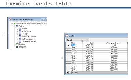
Now examine the Events data table. Contrasted with the Inspections table, its information represents the other side of the coin. Both Event and Inspection data are required for CBM optimization. The EXAKT modelling process is one of correlation of Events (of all kinds) and Inspections (that is, condition data). Condition data often comes from specialized databases provided by CBM product or service vendors. Common examples are oil analysis and vibration analysis. These databases are invariably well organized and consistently populated.

The Events data, on the other hand, often comes from the organization’s CMMS (computerized maintenance management system) and from production databases. (The records in the CMMS, typically, have been less rigorously kept than the others. Hence EXAKT contains tools and techniques to validate and get the CMMS data into shape.) The basic required Events are: 1) Beginning (an item has been placed into service) designated by B. 2) Ending by Failure, (EF)and 3) Ending by Suspension (ES). By “suspension” we mean that the item has been taken out of service for any reason other than failure. For example, it may have been preventively replaced.

Once again the Ident, Date of the Event, WorkingAge are required fields. The Event itself is recorded in the fourth column. “OC” in this example represents an “oil change” event. Any event which affects the condition data (in this case it would initialize the wear metals and contaminant elements to zero) must be included in the model.

Examine the other tables

CovariatesOnEvent , X

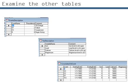
Examine the CovariatesOnEvent . We must provide the “initialization values” for each event. Note that in this case we are initializing wear metals and contaminants to zero and additives to their new-condition levels. We may also establish calendar periods for which these initialized values to be used. (For example, the brand or grade of lubricating oil may be changed periodically.)

EventsDescription, X

Examine the EventsDescription table. The column “Precedence” tells EXAKT program in which order to consider separate events that occur at the same date/time. For example, if an oil sample is drawn from an oil drain, we would wish that the sequence of the Inspection precede that of the oil change. The inspection event is implicitly given the precedence “0”.

VarDescription, X

Examine the VarDescription table. The variable name can contain the symbol or text associated with some feature of a time series, Fourier transform, or in this case, an atomic emission spectrum. Finding features that reflect the state of a failure mode is the purpose of techniques generally called “signal processing”.

Models table

Models, X

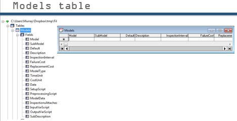
Examine the Models table. It contains no records yet. That is because you have not yet begun building a model. This table is populated automatically by EXAKT as you proceed. The only time you might access this table manually would be to delete certain sub-model(s) that you do not wish to retain. A sub-model is one of any number of models that are tested in the modelling process. The sub-model that is considered the best, is then exported. An agent will use to provide optimized decision support based on a particular item’s current condition data.

Enter general project data

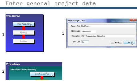
Now that we have examined the internal and external database tables we are ready to proceed with the development of a  CBM optimization model. We turn our attention to the right hand window pane containing buttons arranged in a flow chart of activities. We enter the general project data using these steps:

Data Preparation,
Enter General Data,
Project Title: Haul Trucks,
CBM Model: Trans Oil Anal,
Description: 350 T Transmission Oil Analysis,
Time Unit: Hrs., OK.

Combine the Events and Inspections tables into the C_Inspections table

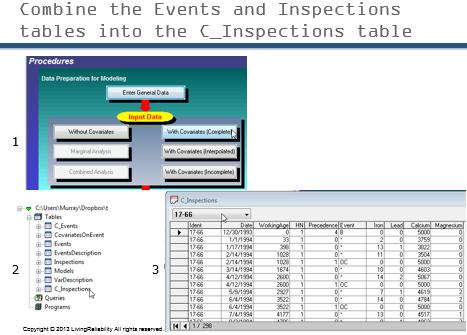
Next we instruct EXAKT to assemble the Events and Inspections into a single (virtual) table called C_Inspections . The algorithm will use this table for subsequent RA calculations. There are a number of alternative buttons we may hit at this point. For this exercise please hit

With Covariates (Complete).

If the With Covariate (Complete) button is not activated, open and close a table on the left. After hitting this button two more tables will appear in the left pane, C_Events and C_Inspections.

C_Inspections , X

Examine the C_Inspections table. Note that the records of both tables (Events and Inspections) have been combined and arranged in chronological order in the single table C_Inspections . Inspection (condition monitoring) record events are designated by an *. The other event records (B, EF, ES, OC) have monitored data (covariate) values set to their initialized levels according to the CovariatesOnEvent table discussed previously.

Build a trial model with all four CBM variables

Now let’s begin the “modelling” phase of the analysis.

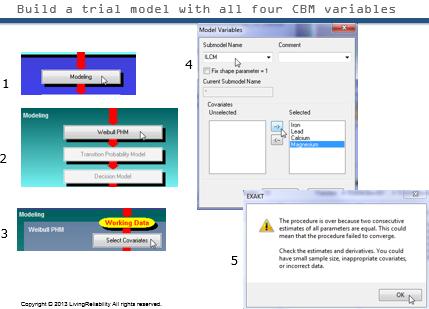
Modelling (button on flow diagram),
Weibull PHM, With
Select Covariates,
Submodel Name: ilcm,
Covariates Unselected: Iron, -> -> -> ->
OK, OK (in warning message), X.

After executing the above steps, the Trans Oil Anal (ilcm) report window appears.

Examine the parameter estimation report.

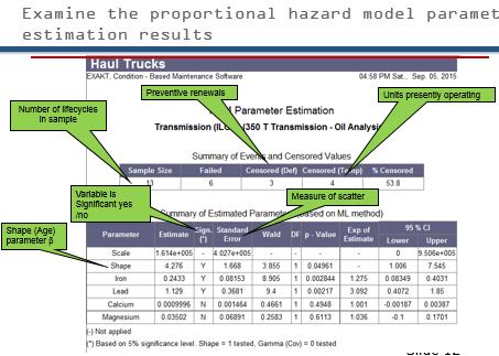
The “Summary of Events and Censored Values” presents the overall summary of the data being analyzed. A “Sample Size” of 13 means that there are 13 histories or lifetimes having a beginning and some kind of ending event.

Of the 13 histories 6 ended in failure, 3 (Censored (Def)) ended prior to a failure, and 4 (Censored (Temp)) units are currently in operation at the time of building this model. They are referred to in EXAKT as “temporary suspensions” and are identified automatically by the software. The next tabulation “Summary of Estimated Parameters” provides the results of our first sub-model “ilcm”. The column whose heading is “Sign.” indicates whether a “Parameter” shape β, or covariate parameter γ_i is significant – that is, whether it has been found to be statistically related to failure.

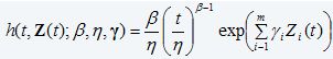
The Shape (i.e. WorkingAge), Iron, and Lead are designated as significant (at this point in the analysis) while Calcium and Magnesium are not. Note that Magnesium has the highest Wald Test p-Value. (The Wald Test is used to test if an independent variable has a statistically significant relationship with a dependent variable. The p-value represents the relative probability that Magnesium has no significant impact on risk of failure). The software estimates the parameters have been estimated numerically in the PHM model:

Build PH model with all significant variables

The next step is to try a different model by eliminating the variable whose impact on the probability of failure is lowest – it is magnesium.

Close the PHM Parameter Estimation report window and execute the following steps in order to create 2 more sub-models:

Select Covariates, sub-model Name: ilc, Magnesium, ← OK , X
Select Covariates, sub-model Name: il, Calcium, ← , OK, OK  (in warning message), X

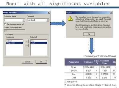
Notice that we are successively removing the covariate with the highest reported p-Value. After hitting (the first) “OK” you will receive an alert warning message from EXAKT.m telling you that the procedure is over. This is normal for samples of small size (low number of histories ending in failure). You may safely ignore this message by hitting OK in the message box.

The columns in the reports provide the results of various statistical tests. They are well-explained in the Exakt Manual. The manual is accessible from the Windows Start menu or from the help menu.

Eliminate a significant variable

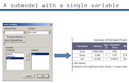
At this point we have a sub-model with covariates and shape parameter that are all significant. We may conclude that this, therefore, is potentially an acceptable model for failure risk prediction. To be rigorous, we should test one last possible combination – a sub-model with iron alone. (We choose Iron as it is the variable with the lowest p-value and thus is likely to have the strongest relationship to failure.)

Select Covariates,
sub-model Name:
i, Lead, ←,
OK, OK  (in warning message), X

The report tells us that this is also a potentially good predictive model (i.e. iron alone is still significant). In the next step we decide which of the two sub-models (i or il) should be retained and ultimately deployed in the decision agent.

Compare the two models

Execute these steps:

Comparative Report,
Compare: il, (Compare the more complex model with the simpler model)
i, →, OK, X

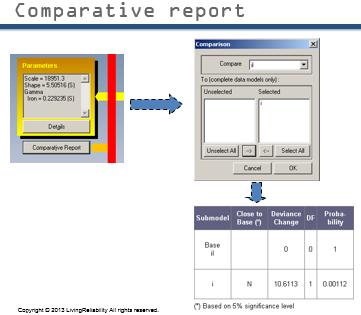
The “PHM Parameter Estimation – Comparison” report is displayed. The “N” in the second column is telling you that the sub-model “i” is not close to the base sub-model “il”. This means that this simpler sub-model is not as good as il. That is, the il model contains significant information that is not present in the i model. We would be losing confidence by using it rather than the more complete model “il”.

 

Reactivate the model to be retained

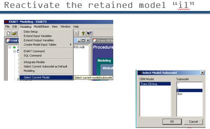
In this step we examine the results of statistical testing performed by EXAKT on the retained sub-model, il. Reactivate this model with the following steps:

Activate left (Transmission_ WMOD.mdb) pane.
Modeling (menu bar),
Select Current Model,
Sub model: il,
OK.

Notice that the Model (Trans Oil Anal (il) appears in the title bar of the flow chart window.

Goodness of fit

Now hit the Modeling button (not the Modeling menu item).

Modeling , Summary Report

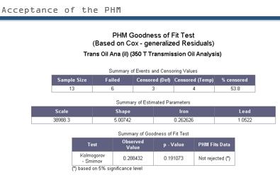
The table “Summary of Goodness of Fit Test” report tells us that the proportional hazards model we constructed for risk as a function of working age and the two significant covariates “fits” the data well enough for it to be used with a confidence of 95%.

The test used for this is known as the Kolmogorov Smirnov test and is well accepted as a statistical tool. The test shows that the model is not rejected at the 5% significance level – i.e. it is accepted at a 95% confidence level.

Transition model

Transition Probability Model,
Covariate Bands,
Covariate: Lead

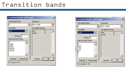
Upon executing the above steps of we see that EXAKT has created a set of bands (listed under Interval Start Points). These are “transition” states for Lead and Iron. These divisions or bands are used by the software to build a “transition probability model”. The transition probability model calculates the probability of jumping to another state within the next inspection interval. (An example of what we mean by jumping to another state will be given below.

select Covariate Iron

Notice the transition bands provided for Iron are quite different than those of Lead. This is because historical iron measurements are scattered throughout an entirely different range of values. This can be ascertained using EXAKT’s cross-graph function (to be described in another Tutorial, and also discussed in the user guide and manual)

OK

Transition probability matrix

Transition Rates, Display Survival, Working Age: 8000, Observation Interval: 200, Report, Close the report, close the “Display Survival Probabilities” dialog.

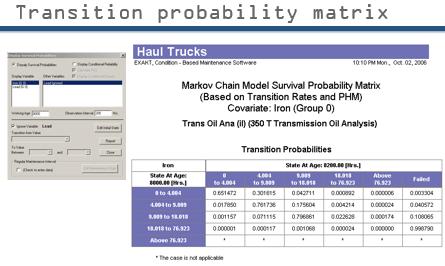
Notice that the two buttons “Display Matrix” and “Display Survival” have become active. Let’s examine the Display Survival function report. Set WorkingAge to, say, 8000 hours, and Observation Interval to, say 200 hours. (assuming, for example, that our asset is currently at age 8000 and we are interested in knowing its risk of failure in the next 200 hours.) The “Markov Chain Model Survival Probability matrix” report is displayed. The probabilities of Iron values jumping to another state and the probability of failure in the upcoming interval are displayed in a tabular format.

(This table represents only a part of the entire set of transition probabilities taken into account by the model. We have chosen to ignore the other significant covariate, Lead in this report. To include more than one covariate in the visual report would require the representation of multi-dimensional matrices. Instead this report allows us to see how a single variable changes irrespective of the others.) Looking at the table we see, for example, that the cell “0- 4.004” and “4.004-9.009” has the entry 0.301615. This means that there is a 30.1615% probability that iron will be in that state at the next monitoring interval. Hence this report provides the probabilities of being in any state at some future time. (Of course, this report is provided for analysis purposes only while building the model. The transition probabilities are fully integrated into the final decision model that will be deployed in section 2.)

Optimal decision policy

Set the decision (business) model parameters

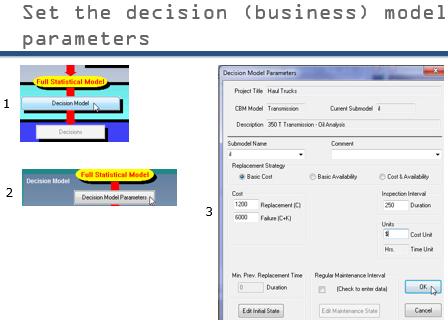
Now for the final step in developing a decision optimization model. We blend into the model the economics governing the failure and repair of this item.

Decision Model,
Decision Model Parameters,
Replacement (C): 1200,
Failure (C+K): 6000,
Cost Unit: $,
Inspection Interval: 250, OK,
Full Report Icon (to the left of the Print Icon), X

We apply the average cost of a preventive repair C and the average cost (including consequential costs) of a failure C+K. (It is rarely necessary to have great precision in these relative costs. The cost sensitivity function of EXAKT (described in the manual) allows us to confirm the adequacy of these cost amounts for the decision model in question.

Cost analysis

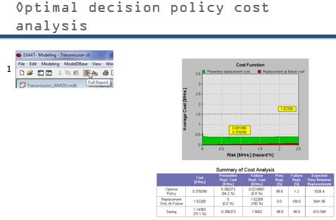
After hitting the Full Report Icon (which you’ll find to the left of the Print Icon on the Tool Bar), the “Condition Based Replacement Policy – Cost Analysis report appears. Examine the “Summary of Cost Analysis” table below the Cost Function graph. It is telling you that by adhering to the interpretive decisions of the model, an optimal long run ratio of preventive-to-failure replacements of 98.8:1.2 will be attained. This policy will result in a cost savings of 75.1% relative to a replacement-only-at-failure policy. (The cost comparison reporting function similarly compares the optimal EXAKT policy with existing practice. It’s usage is described in the EXAKT user manual.)

Testing

We have been, up to now, building a model based on the historical data from the entire fleet. We may now test the model on any individual unit either for the current situation (i.e. the latest data available in the database, called “LH” for last history) or we may look at any other history retroactively.

Decisions, 17-66,
shift+17-79,
Report,
Full Report Icon ,
PgDn, PgDn, PgDn, X,
Last Histories dialog, X

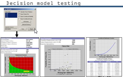
The steps above display the reports of the latest monitored values of each unit. Four sets of graphs are shown – one for each of the four units 17-66, 17-67, 17-77 and 17-79. By examining the graphs we see that none are in alarm at the current moment when this snapshot of the data has been made.

If the weighted sum of the significant covariates (i.e. the y-axis plotted variable) falls in the Green region, no action is necessary; in the yellow, the item should be renewed before the next monitoring interval; in the read, the item should be repaired or replaced immediately. It should be noted that these boundaries vary with working age. This reflects the analysis findings that working age, as well as Iron and Lead, are significant failure risk factors. At some point in the past the values for 17-67 hit the red zone. This may indicate a spurious laboratory result that was corrected in a follow-up verification. (For modeling, known incorrect data should be removed from consideration.) Note that the x-axis scale differs from graph to graph depending on the current age of the unit.

Prepare to export the model

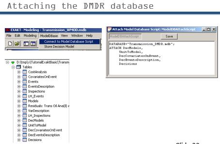
The analysis and model building phase is complete. We are now ready to export the optimal decision model we created into our maintenance system environment (where it has access to continuously renewing data), and, where it can do its job. An empty database has been prepared. Its purpose is to hold all EXAKT decision models and their respective future decision records. In the next slides, we’ll see how the EXAKT decision agent accesses each model and returns the decisions to the database where they may be accessed by the EAM.

Activate the left pane, ModelDbase, Connect to Database Script, key in (or copy) the script for exporting the model

Database="Transmission_DMDR.mdb";
ATTACH DecModels,
UnitToModel,
DecCovariatesOnEvent,
DecEventsDescription,
Decisions

Save

In the next slide we will send the model to a database located on the network. You will notice that several new table links appear in the tree view. Now that the links to the Transmission_DMDR.mdb database have been set up, we proceed to the actual export in the next slide.

Store the the decision model in the DMDR database

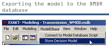
Execute these steps:

ModelDbase,
Store the Decision model,

Close EXAKTm

You may examine the tables DecModels, UnitToModel, DecCovariatesOnEvent, DecEventsDescription (by double clicking on the file names in the tree view of the left pane) to see just what information has been exported to the external database.

Launch the decision agent

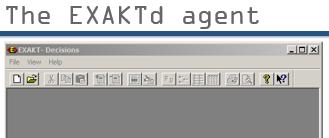
The EXAKTd decision agent operates independently from EXAKTm. You may set it up to run automatically in a Windows scheduled task, or in response to system commands with parameters from other programs. Or, it can be run from its own user friendly interface as described in the following slides. In this section we run the “agent” manually. (It can also be set up to run automatically). After you execute the following steps the user interface of the EXAKTd decision agent appears.

Start, Programs, Exakt, Exakt for Decisions

Create working database

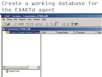
Execute the steps below to create a “working database” for the decision agent to use. (it will be named Transmissions_WDEC.mdb).

File, New, Navigate to your working folder. File name:  Transmission_WDEC.mdb, Create.

 

 

Connect to the DMDR database

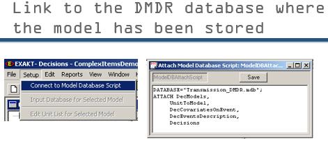
Now we will link to the database where we previously exported our model (Slide 22 of Section I.). After executing these steps you will see the name of the Model you created, “Trans Oil Anal” in the top left pane

Setup, Connect to model database script

copy and paste this script:

Database="Transmission_DMDR.mdb";
ATTACH DecModels,
UnitToModel,
DecCovariatesOnEvent,
DecEventsDescription,
Decisions

Save

EXAKTd for CBM decision action

List units

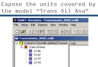
Expand “Trans Oil Anal”

After executing the above step, you will see each of the units whose optimal decisions for oil analysis will be governed by this model. (new units may be added easily in the EXAKTd program.)

 

 

Select a unit

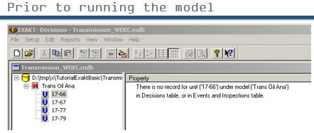
17-66

By selecting any unit in the top left pane, we see a list of properties but no values. Next, we will run the agent manually on the latest available set of condition monitoring oil analysis data.

Run model

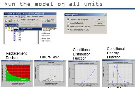
Now you will re-select the Model “Trans Oil Anal” and execute the decision agent by following these steps.

Trans Oil Anal, Reports, Create reports, Calculate time to replace

Cycle through all of the graphics of Slide 30 by hitting PgDn and PgUp

Exception summary report

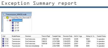
Highlighting  the model name (failure mode) “Trans Oil Anal” displays the summary report  where exceptions may be managed.

 

 

Drill down from the summary report

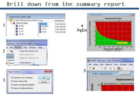
You may select a Unit for full reporting by highlighting it in the summary (1).  Hit Reports, Create Reports (2). Select the report options OK (3). PgDn and PgUp to scroll through the various reliability analysis graphical representations for that unit (4). Display the full report (5).

 

Full decision reports

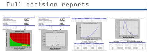
The full decision reports provide the detailed information regarding the unit including the actual values of the condition data, the cost analysis, predictive confidence, current working age, significant variable transitions, conditional failure probability, density, standard deviation, confidence intervals, and Remaining Useful Life Estimate (RULE).

Custom reporting

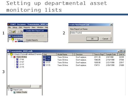
The normal use of EXAKT CBM decision reporting would be via the EAM system accessing and filtering the records in the Decisions table of the _DMDR database. Nevertheless basis reporting, say by department, can be done directly via the Exaktd agent program. For example, say there are two departments called “Indoor Trucks” and “Outdoor Trucks” under responsibility of two different superintendents. Each may have his own customized report by copying the respective units in the summary table to their respective lists. This is shown in Slide 35.

Manage units by department

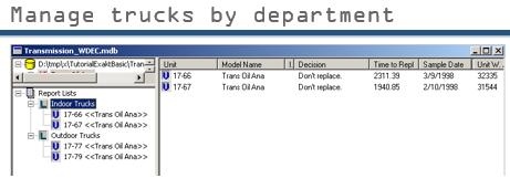
Using the Exaktd decision agent program for reporting is simple. The manual should be consulted for running the decision agent automatically at regular so that the EAM contains the most up-to-date prognostics.

N.B. (Important note)

The entire exercise above, onerous as it appears, can be executed in less than ten minutes, once you gain some familiarity with the user interface.^[1] The mechanics of using the EXAKT program are, in actuality, the easiest part of the CBM decision modeling process. The more difficult part of the process begins with the maintenance work order. Specifically, the work order form wherein the technician enters the right data. The true challenge lies in understanding the nature of data. The type and quality of data required for the above analysis is explained in the article CBM Optimization.

© 2015 – 2021, Murray Wiseman. All rights reserved.

1. ^[1]which can be achieved by repeating the exercise 2 or 3 times.↩