We all believe or we suspect that data is the key to the way forwards – i.e. the quality, type and timely input into a software program will turn out optimal inspection frequencies and other types of maintenance decisions.
More specifically, there are two broad categories of data needed for analysis and decision modeling:
- Condition monitoring (CM) data encompassing everything observed in the operating machine at regular age intervals. This usually includes sensor data, oil analysis data, and vibration analysis data, and
- Age data also called history data, life data, or life cycle data.
Accurate CM data is relatively easy to acquire, structure, manipulate, and display. There are no difficult CM data issues given today’s excellent tools and technology. Accurate age data on the other hand presents a major obstacle. We extract age data from the CMMS. Therein lies the problem. One issue is that for purposes of analysis we need to distinguish failure from suspension. A suspension is a failure mode renewal for any reason other than failure. Current CMMS and RA procedures don’t provide data adequate for RA (Reliability Analysis) and decision modeling.
In various articles we delve into detail on the actual data requirements and precisely how typical data inadequacies affect predictive confidence in virtually all maintenance organizations. Below we include some of the discussion.
The transitions between one equipment health state to another are represented using a method such as the Markov Failure Time model, combined with a model of the “conditional” failure probability v.s. the equipment age v.s. its Condition Monitoring (CM) data. The applied model will provide a remaining useful life estimate (RULE) at the granularity of interest, say at the subsystem, component, or failure mode (part) level.
But what is exactly happening mathematically. Can we provide what we would call an idiot’s guide to this? Certainly, here is the “idiot’s” guide.
The EXAKT CBM Model
Given the scale of maintenance in a mining or energy related operation, it is desirable that the process for making a CBM decision be optimal, automated, and verifiable. The following describes a CBM optimizing system called EXAKT. CBM Decision Model (DM) construction is illustrated below in Figure 1. Although the Reliability Analysis (RA) modeling illustrated in the figure and described in the following paragraphs appears complicated, it is, in fact, quick and easy thanks to software.
The infinitely more difficult part of developing optimized Decision Models (DMs) is the procurement of the right data from the CMMS historical records. Only a LRCM (Living RCM)) process can routinely feed the right data to RA (Reliability Analysis) for the development of optimized and verifiable DMs.
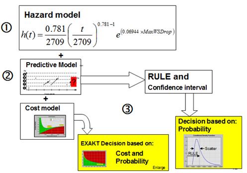
The modeling process labeled 1, 2, and 3 as illustrated in Figure 1 consists of the following three phases:
- The first phase develops the reliability model. An example of a reliability model is seen in the top left block of Figure 1. The equation is known as a “Proportional Hazard Model (PHM)” with Weibull baseline wherein:
- h(t) is the Failure Rate function.
- The first factor on the right hand side
 is recognizable as the Weibull Failure Rate where (in this example) the shape parameter β is 0.781 and the scale parameter η is 2709.
 - The second factor on the right side
 extends the Weibull failure rate equation to include relevant CBM data. Each CBM variable is multiplied by a vector parameter γi. In the simple example with only 1 relevant CM data variable, γi = 0.06944. The parameters β, η, and γi are estimated by a numerical algorithm applied to a sample of life cycles and concurrent CBM data. The product of each significant CBM variable and its γi are summed within the exponential term. In the example equation we see that age t is significant since β is different from 1. If β were equal to one the factor
  would become 1 and the failure rate would then be independent of age and dependent only on the significant CBM (i.e. CM data) variables. This is a desirable CBM situation. If, in addition to a low value of β, the confidence in the model is high (see Phase 3 below) then our maintenance decisions based on CBM data will be optimal ones. CBM decisions when optimized will yield lower overall cost and higher availability than Time (Age) Based Maintenance (TBM) decisions. In the example, only one condition monitoring variable MaxWSDrop appears in the exponential term. It is significant since its γi is found by the software to be significantly different from zero.
- In the second phase of CBM modeling we build a prediction model (middle block on the left side of Figure 1). A combination of value ranges[1] of the significant variables constitutes a “state”. If there are two significant variables and each has 3 discrete levels then transitions could occur among 9 states. Past transitions from one state to another form a probability history in the form of a probability matrix that is used to predict the likely future states of the variables.[2]
- Finally the reliability and predictive models (the foregoing Phase 1 and 2) are combined in the third modeling phase to generate a Remaining Useful Life Estimate (RULE). Confidence in the estimate can be expressed, for example, as a standard deviation. The RULE and its confidence (scatter) are illustrated in the “Conditional Probability Density” graph in the bottom left block of Figure 1.The reliability and predictive models may be combined with business factors to develop a “Cost model” an example of which is shown on the left of Figure 1. The vertical axis represents the overall cost of maintaining the component. The Horizontal axis measures “Risk”. The low point on the graph indicates the optimal risk. It is the level of risk that results in the lowest maintenance cost, the highest availability, or the highest profitability depending on the optimizing objective that the Reliability Engineer sets into the model.The optimal DM is represented by the green, yellow, and red graph at the bottom of the Figure 1. The vertical axis measures the weighted sum of the CBM significant variables. The horizontal axis measures the working age of the asset. If the weighted sum of significant variables falls in the red region of the graph, a Potential Failure (PF) is declared tentatively subject to confirmation at the time of work order execution. Each point on the crossover boundary to the red area corresponds to the optimal risk as calculated as the low point on the Cost model graph of Figure 1.
You can try a couple of exercises at http://www.
- [1]Consecutive value ranges making up the total range of the values of Iron dissolved in lubricating oil may, for example, be: <10 ppm, 11-20 ppm, 21-50 ppm, and >50 ppm. Ranges are determined for the other predictive variables. The combination of value ranges attained by each variable at a given time defines a “state”. The predictive failure time algorithm calculates the probability of the occurrence of every possible future state.↩
- [2] http://www.livingreliability.
com/en/posts/the-elusive-p-f- interval/ describes the transition model more fully.↩