CBM Optimization

Nature, and therefore humankind, must optimize to survive and prosper. Each species in the animal kingdom strives for the best long term results of its actions. Whether divinely designed or as a result of natural selection, activity is calculated (optimized) to balance low energy expenditure with maximum caloric intake. No less true is a business’s need to optimize, if it is to compete in the global jungle for its very survival. Companies that offer better goods and services at lower cost survive better in the marketplace and tend to accumulate an ever-growing market share. Poorly-adapting companies will be forced out by better-adapting ones: “killed” by the competition.

We gather information in maintenance as a precursor to decision making and action. A policy or “model” is a procedure  for making decisions in the face of facts. Achieving value from a decision policy depends on:

1. Having the right data, and
2. Transforming that data into the correct (best) action.

1. The right data

This slide presentation divides data into two major categories, and a number of sub-categories. By understanding the nature of maintenance related data, Reliability Engineers will collect and analyze the “right” data.

LRCM is a process that ensures the right data is used for designing maintenance decision policies. Those policies will be applied day-to-day to make the optimal decisions that will achieve the enterprise’s long run objectives.

2. Optimal CBM Decisions

The principle of EXAKT

Figure 1 Two decision paths in EXAKT

The flow diagram of Figure 1 illustrates two ways of deciding whether an item, component, or failure mode is in a Potential Failure (P) state.  The two decision processes can be categorized as:

1. An optimal decision based on the combination of failure probability and the quantifiable consequences of the failure (Path 1), and
2. A decision based solely on failure probability (Path 2).

The first CBM decision making strategy will support decisions related to operational and non-operational consequences of failure whose economic impact can be quantified, for example, the failure of a component in a production line. The second method will apply to decisions that must be based strictly on probability. These include situations beyond the expected, whose failure costs are unknown or incalculable, such as where catastrophic environmental, health, and safety consequences are concerned. Managers use both types of decision methods regularly within the compass of their responsibilities. This article will describe the optimal decision process based on business factors combined with failure probability.

Cost minimization review

The top graph of Figure 2 plots the hazard rate (also called failure rate). It is the probability of an item failing at any  instant given that it has survived to that point in time.

Figure 2 Hazard and Cost Graphs

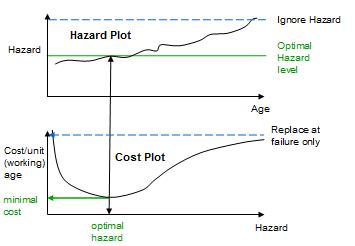
Hazard may change in time as a result of many factors. We ask these questions, in forming our decision policy, “At what hazard level should we intervene?” “Should we ignore hazard altogether, or should we act when the hazard reaches  some specific value?”

The bottom graph of Figure 2 recognizes that an enterprise’s profit and loss statement considers good performance as being low cost per unit of production (working age). Therefore, we would wish to choose a hazard level intervention point that results in lowest cost. Intuitively, we surmise that a policy of operating at very low hazard will be expensive (as illustrated on the left extremity of the cost plot). On the other hand, choosing to operate at a very high hazard rate will ignore hazard and incur the costs of running to failure. We conclude that there will be a best policy somewhere between the two extremes. Hence the cost curve will be trough-shaped (as illustrated) when plotted against the operating hazard rate. Our objective is to find the optimal hazard level that corresponds to the low point on the curve, resulting in minimal overall cost.

To apply the optimal CBM decision modeling procedure the Reliability Engineer (RE) will need to discover how hazard varies with observed operational and condition monitoring data. He finds such a relationship by estimating the parameters of the Proportional Hazard Model (PHM).^[1]

EXAKT’s basic cost model

The Reliability Engineer, upon establishing the relationship among hazard rate, age and relevant condition indicators, enters the required business information into the form shown in Figure 3.

Figure 3 Decision model parameters for cost minimization

The software finds the CBM and age control limits that, if acted upon consistently by the maintenance department, will result in lowest overall maintenance costs. The optimal decision model is found by minimizing the cost function:

Where:
C_E is the total expected cost per unit of working age of maintaining the asset (Item, Failure Mode)
Q is the failure probability
W is the working age at renewal
C is the cost of the preventive maintenance action.
K is the penalty cost of failure.

EXAKT bases its cost model on the user supplied average cost of a functional failure and the average cost of a preventive action.^[2] In this simplest of the EXAKT optimization procedures, the analyst provides the costs (e.g. materials, labor, lost production), “C”, of planned maintenance and the added economic impact (e.g. materials, labor, lost production, secondary damage to equipment or the environment), K, as a result of the unplanned nature of the functional interruption.

Figure 4 Cost Function Graph

The results of the optimization are shown, as an example, in the graph^[3] of Figure 4 and in Table 1.

Any cost value on the curve consists of a red portion, attributable to unplanned failures, and a green portion, representing the average costs associated with preventive maintenance.
Table 1 summarizes the information in the graph. It compares the optimal cost ($94) and optimal mean time between asset renewals (863 d)) of the optimal policy with those ($168 and 1138 d) of the “run-to-failure” policy. It quantifies the expected preventive and failure costs ($57 and $37 respectively) and the percentage of incidences (83.5% will be preventive actions and 16.5% will be instigated by a failure) achieved when adhering to the optimal policy.

Table 1

The table’s content illustrates that the optimal policy will cause us to intervene more often on the average (863 versus 1138 days), in order to achieve a net per unit saving ( of $74 or 44%).

The foregoing described CBM optimization for the objective cost minimization. Subsequent pages and sections discuss the theory and procedures for the optimization of CBM programs with the objectives of achieving maximum availability or maximum profitability (accounting for both cost and downtime).

© 2011 – 2015, Murray Wiseman. All rights reserved.

1. ^[1]The  step-by-step PHM procedure can be found from the Sidebar under Categories | CBM | Exercises | Exercise 1. The PHM description can be found under Categories | CBM | PF Interval | The Elusive PF Interval↩
2. ^[2]Often managers or engineers do not know in precise terms what the average penalty losses due to failure are. But they usually have a good idea. Fortunately in most cases highly precise differential cost data is unnecessary. Usually ballpark informed estimates will do. In those cases where the estimate error will affect the optimal CBM decision solution the software provides a “sensitivity” analysis to alert the user to the need to acquire a more accurate penalty to cost ratio. ↩
3. ^[3]The vertical axis is the cost of preventive plus reactive maintenance per unit of operation, for example tons of ore hauled. The horizontal axis is the risk defined as the hazard rate (aka failure rate) × the penalty K for failure.↩