The elusive P-F interval

CBM decisions based on economics and probability

Successful businesses confronted with a variety of risk factors, optimize their policies and resources in order to achieve their ultimate objectives. An economic decision model is a rule for preventive renewal of an asset that minimizes the average per unit cost associated with maintenance (proactive and reactive) over a long time horizon. (This cost is the key performance indicator most directly related to shareholder value.) Such a rule for CBM may be reasonably expressed as a control-limit policy. If T is the actual failure time: perform preventive maintenance at T_d, if T_d < T; or perform reactive maintenance at T if T_d ≥ T, where

T_d=inf{t≥0:Kh(t,Z^(d)(t))≥d} (eq. 10)

K is the cost penalty associated with functional failure, h(t,Z^(d)(t) is the hazard, and d (> 0) is the risk control limit for performing preventive maintenance. Here risk is defined as the functional failure cost penalty K times the hazard rate.

The long-run expected cost of maintenance (preventive and reactive) per unit of working age will be

(eq. 11)

where C_p is the cost of preventive maintenance, C_f = C_p+K is the cost of reactive maintenance, Q(d)=P(T_d≥T) is the probability of failure prior to a preventive action, W(d)=E(min{T_d,T}) is the expected time of maintenance (preventive or reactive).

Let d* be the value of d that minimizes the right-hand side of Equation 11. It corresponds to T* = T_d*. Makis and Jardine in ref. 3 have shown that for a non-decreasing hazard function h(t,Z^(d)(t), rule T* is the best possible replacement policy (ref. 4).

Equation 10 can be re-written for the optimal control limit policy as:

T*=T_d*=inf{t≥0:Kh(t,Z^(d)(t))≥d*} (eq. 12)

For the PHM model with Weibull baseline distribution, it can be interpreted as (ref. 2))

(eq. 13)

where  (eq. 14)

Ref. 2 mentions the numerical solution to Equation 13, which is described in detail in (Ref. 7) and (Ref. 8). The function

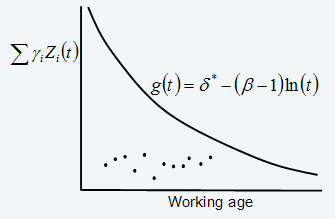
g(t)=δ^*-(β-1)ln(t) (eq. 15)

is the “warning level” function for the condition of the item reflected by a weighted sum of current values of the significant CM variables (covariates). A plot of function versus working age can be viewed as an economical decision chart which shows whether the data suggests that the item has to be replaced.

An example of a decision chart with several inspection points can be found in Figure 3. Detailed case studies based on the model discussed in this section can be found in ref. 5 and (ref. 6).

Figure 3: Sample economical decision chart (for β>1 )

The above development from (ref. 2) speaks to cost as the optimizing objective. Analogous developments have been made in EXAKT considering availability and profitability as optimizing objectives. For these two objectives, we only need to change the objective function in Equation 11 accordingly.

Specifically, for the availability objective, Equation 11 will be replaced by the availability function, defined as the ratio of uptime to the uptime plus the downtime.

where W(d) is the expected uptime, t_p is the downtime as a result of planned maintenance and t_f is the downtime as a result of maintenance forced by a functional failure. The objective is also changed to maximize Φ(d), i.e., d* will be the value of d that minimizes the right-hand side of Equation 16.

For the profitability objective, Equation 11 will be replaced by the global cost function

where a_p is the cost per hour of planned down time and a_f is the cost per hour of unplanned down time. The objective is to minimize Equation 17, i.e., to find d*, which is the value of d that minimizes the right-hand side of Equation 17.

© 2011 – 2015, Murray Wiseman. All rights reserved.