The elusive P-F interval

Assumptions and models used in EXAKT

The advantage of CBM over TBM as a maintenance strategy is that it accounts for both the age of the item as well as its changing state up until the moment of decision making. We assume the item’s state of health is to be encoded within measurable condition indicators (which, of course, is the underlying premise of CBM).

The item’s monitored indicators may be presented as a vector of time dependent random variables, Z(t).

Z(t) = (Z₁(t), Z₂(t), … , Z_m(t)) (eq. 1)

Each variable in the vector contains the value of a certain measurement at that moment. We consider Z(t) a “process” because it changes with each set of CBM readings acquired at regular intervals of time t. Furthermore, it is a stochastic process. A stochastic process is sometimes called a random process. Unlike a deterministic process, instead of having only one possible ‘reality’ of how the process might evolve with time, in a stochastic process there is some indeterminacy in its future evolution. This uncertainty is described by probability distributions. There are many possibilities of where the process might go, but some paths are more probable than others. Z(t), then, is said to be an “m-dimensional stochastic covariate process” observed at regular intervals of time, t.

We let T, a random variable, represent the failure time of the item. A primary goal of CBM is to predict T given the current age t and the current measurements of Z(t). Achieving this goal will require us to develop a statistical model that combines the stochastic behavior of the CBM readings Z(t) with a model for the hazard rate as a function of age t and the current CBM readings Z(t).

Of particular interest to us in accomplishing this objective are two theoretical models:

1. the Cox proportional hazards model (PHM) with time-dependent covariates for describing the failure behavior, and
2. the non-homogeneous Markov failure time process for describing the evolution behavior of the covariate process.

In this article we will show how these two models may be combined for the predictive purposes of CBM.

Proportional hazards model with time-dependent covariates

In EXAKT the influence of condition monitoring (CM) indicators on the failure time is modeled using a Proportional Hazards Model (PHM). First proposed by Cox in 1973 (Cox D.R., Oakes D., 1984.), the Cox PHM and its variants have become one of the most widely used tools in the statistical analysis of lifetime data in biomedical sciences and in reliability. The specific model used in EXAKT is a PHM with time-dependent covariates and a Weibull baseline hazard. It is described by the hazard function:

(eq. 2)

where β>0 is the shape parameter, η>0 is the scale parameter, and γ =( γ₁,γ₂,… γ_m,) is the coefficient vector for the condition monitoring variable (covariate) vector Z(t). The parameters β, η, and γ, will need to be estimated in the numerical solution.

Markov failure time process

The physical CBM measurements of each Z_i(t) will fall into classes or states that we have set up and labeled as, for example, “new”, “normal”, “warning”, or “danger”. These designations (a common practice in CBM) constitute the state space of the stochastic process Z(t). As such, the covariate vector Z(t) can be reasonably discretized to reflect, meaningfully, each of its states. Specifically, we discretize the range of each covariate Z_i(t) into a finite number of intervals each of which has a representative value. This value can be taken as any value in an interval’s range. EXAKT takes the midpoint of each interval as the value representing the condition indicator’s state.

Define the discretized covariate process Z(t) as Z^(d)(t) = (Z₁^(d)(t), Z₂^(d)(t), … , Z_m^(d)(t)).

such that the value of each Z_i^(d)(t) is equal to the representative value of the interval into which Z_i(t) falls.

Denote all possible values (states) of Z^(d)(t) as R₁^(z), R₂^(z), …, R_n^(z)

where R_i^(z) = (R_i1^(z), R_i2^(z), …, R_im^(z)) is a representative value of the covariate Z_j^(d)(t).

R_i^(z) represents the i^th state of the discretized covariate process Z^(d)(t).

We predict likely future states of the discretized process Z^(d) (t), by endowing it with some kind of probabilistic behavior. A non-homogeneous discrete Markov process has been shown (Bogdanoff & Kozin, 1985; Kopnov & Kanajev, 1994; Pulkkinen, 1991) to model the stochastic behavior of time dependent condition monitoring variables related to wear propagation.

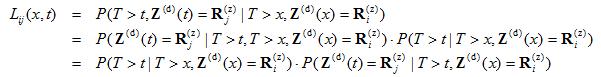
In EXAKT, it is assumed that Z^(d)(t) follows a non-homogeneous Markov failure time model described by the transition probabilities

L_ij(x,t)=P(T>t, Z^(d)(t)= R_j^(z)|T>x, Z^(d)(x)= R_i^(z)) (eq. 3)

where:
x is the current working age,
t (t > x) is a future working age, and
i and j are the states of the covariates at x and t respectively, and
T is the time of failure.

The above expression for the transition probability from state i to state j can be read as follows: It is the probability that the item survives until t at which time the state of Z^(d)(t) is j, given that the item will have survived until x when the previous state, Z^(d)(x) was i. The transition behavior can then be displayed in a Markov chain transition probability matrix, for example, that of Table 1.

Table 1 Example of transition probability matrix for one variable at a given state

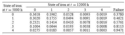
Table 1 can be read as: given that Iron is in State 0 at 5000 h, the probability of remaining in state 0 at 12000 h is 0.3618. The probability, if in state 1 at 5000 h of transiting to state 3 at 12000 h is 0.0091. And so on.

Calculation of the transition probabilities

EXAKT combines the Cox PHM with the Markov failure time model described above. For the following analysis it is convenient to represent Equation 3 in the following form:

Lij(x,t)=P(T>t|T>x, Z^(d)(x)= R_i^(z))) • p_ij(x,t) (eq. 4^[1])

where p_ij(x,t)=P(Z^(d)(t)= R_j^(z)| T>t, Z^(d)(x)= R_i^(z)) (eq. 5)

is the conditional transition probability of the process Z^(d)(t).

For a short interval of time, values of transition probabilities can be approximated as:

L_ij(x,x+Δx)=(1-h(x,R_i^(z))Δx) • p_ij(x,x+ Δx) (eq. 6)

Equation 6 means that we can, in small steps, calculate the future probabilities for the state of the covariate process Z^(d)(t). Using the hazard calculated (from Equation 2) at each successive state we determine the transition probabilities for the next small increment in time, from which we again calculate the hazard, and so on.

CBM decisions based on probability

The “conditional reliability” is the probability of survival to t given that

1. Failure has not occurred prior to the current time x, and
2. CM variables at current time x are R_i^(z)

The conditional reliability function can be expressed as:

(eq. 7)

Equation 7 points out that the conditional reliability is equal to the sum of the conditional transition probabilities from state i to all possible states. Once the conditional reliability function is calculated we can obtain the conditional density from its derivative. We can also find the conditional expectation of T – t, termed the remaining useful life (RUL), as

(eq.8)

In addition, the conditional probability of failure in a short period of time Δt can be found as

(eq. 9)

For a maintenance engineer, predictive information based on current CM data, such as RUL and probability of failure in a future time period, can be valuable for risk assessment and planning maintenance.

© 2011 – 2015, Murray Wiseman. All rights reserved.

1. ^[1]↩