When to maintain? (Slides)

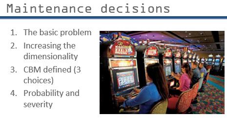
In the casino hall that we call “maintenance” we are faced with choices. Risk is associated with each decision we take. We might say that maintenance is the art and science of managing risk. The choices we make day to day affect the organization’s bottom line profitability. Pursuing the casino metaphor a physical asset might be thought of as a slot machine. The gambler decides whether he should feed his coin into the slot.  Analogously, the maintenance planner decides whether to devote resources to a particular equipment unit. Should he intervene now, next week, or should he defer the decision until he has more information? Does the prize and its probability justify the risk? What are the rules more of the game?

The basic problem

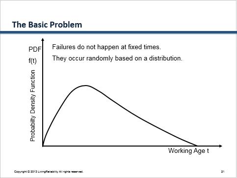
Regardless of which of the six RCM failure patterns governs the failure behavior of a part or failure mode, we do not know the age at which it will fail. The slide asserts that failures do not occur on a fixed schedule. Rather a failure occurs randomly, albeit according to a probability distribution, that will resemble one of the six patterns (A-F)^[1].

Reliability attributes

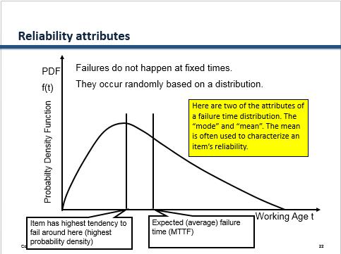
A common measure of reliability is the Mean Time To Failure (MTTF). It can be calculated from the probability distribution. We show in the TBM discussion that, given the ages of failure and preventive renewal, we can easily draw this graph^[2] and extract the MTTF. But how does that help us? If we conduct maintenance say at the expected life, we will have agreed to accept the failures represented by the entire area under the density curve up until that age. That would be 63% in the case of random failure behavior. ^[3]

Can the probability distribution be known exactly?

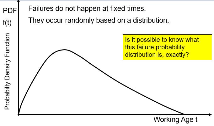
Can we know exactly the failure probability distribution of an item? At first we might answer “no”. After all failures do not happen on a schedule.  Yet upon reflection although we cannot know exactly when failure will occur, we can know exactly the failure’s probability distribution. This way of thinking allows us to change our understanding from determinism to probabilities. The next slide illustrates this notion.

Yes, if we have a data sample

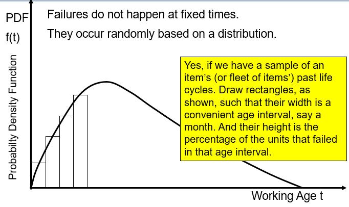
Assume that we have a number of work orders recorded in our EAM. From the work order database we can extract a list of the instances of failure and their respective ages at failure. This information would constitute our “sample”. A sample represents the the general failure behavior of the item. The slide illustrates one way to convert the data sample into a probability distribution.

Still, how does that help?

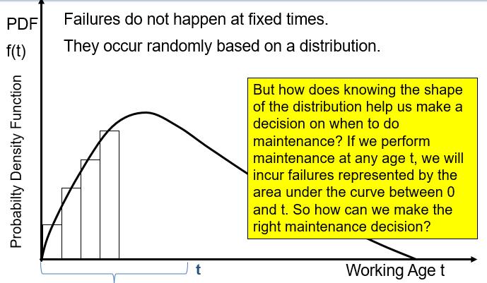
But how does knowing the exact shape of the distribution help us make a decision on when to do maintenance? If we perform maintenance at any give age t, we will incur failures represented by the area under the curve between 0 and t. How can we make the right maintenance decision? The following slides propose a way to circumvent this inherent problem associated with performing maintenance based solely on an item’s age t.

Wide versus narrow distribution

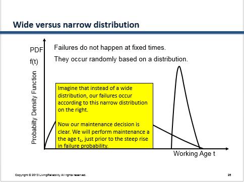
Let’s imagine that the shape of the PDF were not the wide pattern but instead a sharp pattern having a zero probability of failure up until reaching the abrupt rise in probability density as shown? The maintenance engineer’s job would be much easier, would it not? He could schedule maintenance with a high degree of confidence that intervention would take place at the optimum moment.

Real world age based distributions are wide

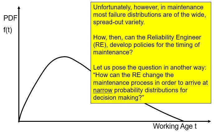
Unfortunately, in the real world, most age reliability failure distributions are of the wide, spread out variety. How then, in view of all the uncertainty reflected by a wide probability distribution, can the Reliability Engineer (RE) develop policies for the optimal timing of maintenance? Let us pose the question in another way. “How can the RE change the maintenance process in order to avail himself of narrow probability distributions for less uncertainty and more confident decision making?” The answer? Introduce relevant dimensions.

Adding a dimension

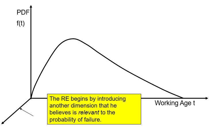
In order to increase the confidence with which to make maintenance decisions the reliability engineer introduces another dimension. The added dimension should add relevant information to the decision process. If the new dimension influences conditional failure probability, then it would narrow the distribution for more confident decision making.

The added dimension must be relevant

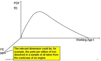
The relevant dimension could be, for example, the parts per million of Iron dissolved in a sample of oil taken from the crankcase of an engine. It is up to the reliability engineer to discover the which indicators are relevant and worthy of being monitored.

 

Example: high iron failures

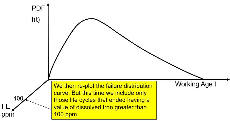
Say we consider in our sample only those items that failed having greater than 100 parts per million of iron dissolved in the lubricating oil. If iron were in fact a significant risk factor we would expect far more failures to occur in that group.

Narrowing the solution

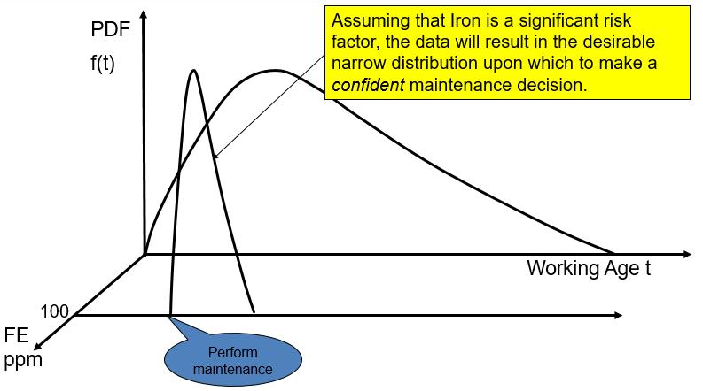
Assuming that Iron is a significant risk factor, and we draw the density curve in the plane located at 100 ppm taking into account only those failures where the iron count exceeds 100 ppm, then we would surmise that the curve will be of the desirable narrow shape and we can make the decision to perform maintenance at the most opportune moment.

It is incumbent on the RE, therefore, to discover influential dimensions for confident maintenance decision making.

Adding significant dimensions (called “condition indicators”) to the maintenance decision making process is the process known as “CBM”.

Formal definition of CBM

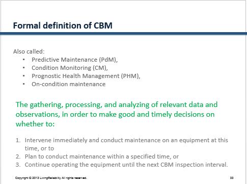
Most maintenance is condition based because most activities are  inspections. The results of the inspections  determine whether intrusive maintenance is required. Often these “preventive” tasks are visual inspections. In the EAM they are called “PM”. Nevertheless they are condition based activities. These PM activities accord entirely with the definition of CBM proposed on the slide. The definition describes the three choices that a maintenance department confronts  over and over again. Given the recurrent nature of the CBM decision it would make sense to establish a rule or policy to respond to the situation. A rule for decision making is called a “decision model”.

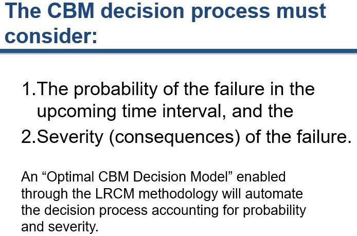
Decision factors: probability of failure and severity of consequences

The importance of CBM was one of the major revelations by the original RCM team working at United Airlines lead by Stanley Nowlan and Howard Heap who submitted their report to the U.S. Department of Commerce on Dec 28, 1978.

1. ^[1]The six patterns of Nowlan and Heap’s RCM study are usually presented as conditional failure probability or hazard h(t) curves. Alternatively the hazard curves may be displayed in the form of probability distributions f(t) by multiplication with the survival probability R(t), i.e. f(t)=h(t)×R(t). Both forms represent the same underlying probability distributions.↩
2. ^[2]it is easy to draw the failure distribution curves precisely as long as we have data in our EAM that accurately identifies the failure modes that occurred and those that didn’t occur but were renewed nonetheless.↩
3. ^[3]See https://www.livingreliability.com/en/posts/what-is-the-scale-parameter/  For non-random failure behavior, for example, for β=2, 55% of items will fail prior to MTTF↩