We have seen that reliability analysis is about counting failure mode instances of failure and preventive renewal. The EAM should be our “counting machine” but, thus far, has not fulfilled that role for the reliability engineer. In these simple exercises we will perform reliability analysis and draw certain conclusions.

Perkins marine diesel engine

Problem background

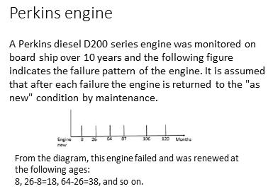
The data shown in Slide 1 tracks six consecutive life times of the engine function on board a ship over 10 years (120 months). From the ship owner’s point of view, the engine ceased functioning for whatever reason. The engine would have been overhauled or replaced with rebuilt unit. In either case it is assumed that it is “as-good-as-new”. When data extends over a long period, for example 10 years, a trend analysis should precede age based (e.g. Weibull) analysis. This will be further explained in the section “Trend Analysis”.

Problem requirements

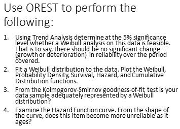
The example illustrates four basic reliability analysis functions for processing age data. First we test whether the data is analyzable in the sense that the asset’s inherent reliability has neither deteriorated nor grown over the period of the sample. This could have occurred as the result of a major redesign or a dramatic change in operating context. In the absence of significant change in reliability we may proceed to fit a Weibull model to the data and thereby learn the relationship between reliability and age. Thirdly a goodness-of-fit test is performed to determine whether the age reliability distribution found adequately represents the data. Finally the resulting graphs may be examined to establish age-reliability behavior.

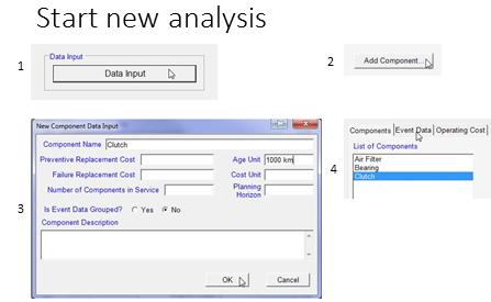
General data

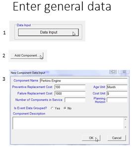
The reliability analysis software, in this case OREST, requires the entry of general data for identifying the item to be examined. A key piece of business information, the cost penalty of failure, is needed to set up  the optimization calculation. In the demo software this information is fixed at 1000 versus 100 for the respective planned and failure renewal costs.

The number of components in service, and planning horizon will be needed later for the spares optimization calculation. We’ll leave these text boxes blank for now.

The application wants to know if the event data is grouped. Data available from the EAM would not be grouped. “Grouped data” refers to events that have already been processed into age groups, for example the number of failures in the age group zero to 1 month, 1 month to 2 months, and so on.

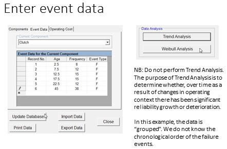
Event data

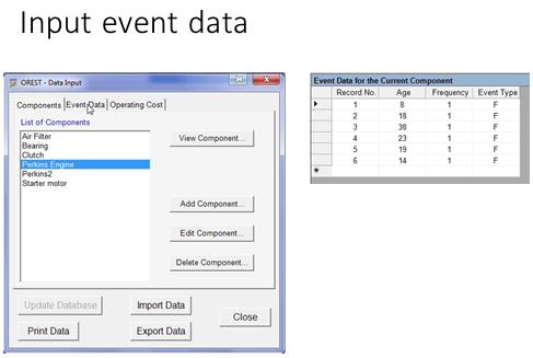
Event data is, by far, the most challenging obstacle to reliability analysis despite the vaunted power of the EAM. What could be more straight forward than recording instances of failure mode events as either having failed or been suspended. Yet this data has eluded reliability engineers and analysts for decades. In this slide we have converted the data from the ten year time line of Slide 1 to individual life data. For example, the first life cycle ended at age 8-0=8, the second at 26-8=18, and so on. In this example all events are failure events. None were preventive renewals (suspensions).

Trend analysis

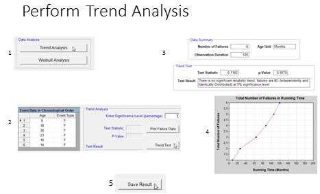
Trend analysis should be performed if the data upon which a Weibull model is to be built extends over a period of time long enough for significant changes to the asset’s inherent to have occurred. In this case the software reports the age data to be “independently and identically distributed” meaning that the upward trend in the graph (Slide 6) of reliability versus running time exhibits no significant deviation.

Weibull analysis

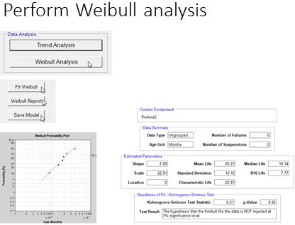
When “clean” Event data is routinely acquired via good EAM work order procedures, Weibull analysis is straight forward and can even become automated within an EAM or APM (Asset Performance Management) reporting system.

 

 

 

Plot the age reliability graphs

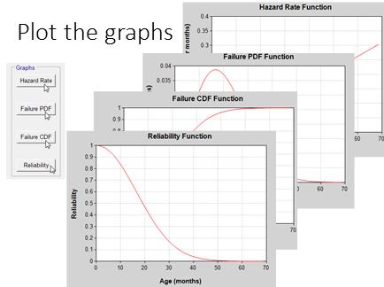
Displaying the age reliability relationship in various graphical forms such as the Reliability (Survival), Cumulative Failure Probability, Probability Density Function, and Hazard (Failure Rate) are equally straight forward.

 

 

 

Clutch assembly failures

Grouped data

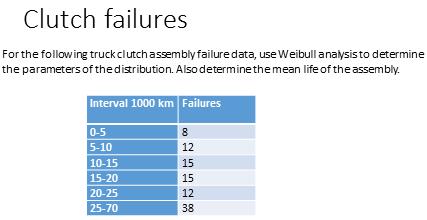
In this example the data has been summarized into consecutive age groups. The number of failures in each age age group is given.

Age is measured in units of 1000 km. As before, we open the OREST software and enter the general data.

Clutch general data

As before enter the general data. For question “Is Event Data Grouped?” we will answer “no” since the software is unable to process grouped data at this time. We will group the data manually.

 

 

 

Clutch event data

To reverse the grouping process we will assume that the items all failed at middle of their respective age ranges. For example in the group 0-5 the mid point would be 2.5, 5-10 7.7, and so on.

We also point out that for grouped data, there is no point in conducting a trend analysis, since there is no chronology given. We have no knowledge of the time period over which the data sample extends. We assume therefore that there would have been no significant growth or deterioration in clutch inherent reliability within the calendar period of this sample.

Clutch reliability graphs and report

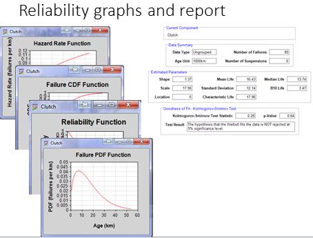
As before, in the software,  graphing and reporting the results of an age based analysis is straight forward. The shape, scale, and location^[1] parameters have been estimated. As well attributes of the distribution such as the mean life, median life, characteristic life, and B10 life have been calculated.

Starter motor example that includes suspensions

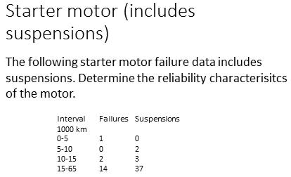
Again the sample of failure and replacement histories is presented in the form of grouped data. Normally, a sample from the EAM database would be generated as individual records for each event.

 

 

Data for starter motor

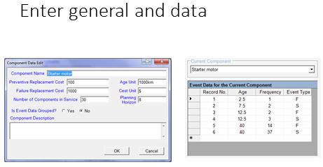
The software requires that separate records be entered for suspensions and failures. Record two at age 7.5 has a frequency of 2 suspensions. While records 3 and 4 capture the failure and suspension frequencies respectively in the third age group of the slide.

Weibull analysis results

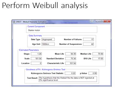
The analysis is performed identically to those of the Engine and Clutch. The results are presented in the Slide.

 

 

 

 

 

 

 

1. ^[1]Sometimes in items which cannot fail at all in the first period of operation, for example grease packed bearings, the curve fitting algorithm will shift the entire distribution to the right by an amount given by the location parameter. The converse may occur wherein a negative location parameter would indicate that the deterioration process will have begun prior to installation, for example chronic problems of damage during storage. ↩