Reliability Analysis: 2 dimensions (Statistical and probabilistic concepts)

Reliability analysis is counting (slides)

Slide 1 Financial analysis is counting money

All types of analysis are about counting in one way or another. The elemental units of information that we count vary with each area of endeavor. Financial analysis is, of course, counting money and categorizing it in a variety of accounts that form a balance sheet or a profit and loss statement.

Reliability analysis (RA) is counting instances of unreliability

Slide 2 Counting instances of failure modes and converting the count to a probability density curve.

Just as the penny is the basic unit of finance it is said that the failure mode is the basic unit of maintenance and reliability. We have seen that the failure mode is the lowest common denominator of RCM – the level at which the effects, consequences, and mitigating tasks are determined. At its most basic RA counts the number of instances of a failure mode that occurred within a calendar window. Dividing that number by the accumulated ages of items at failure approximates the average life or mean time to failure (MTTF). We can go a step further in our counting procedure and graph the relationship between reliability and an item’s age. For a given equipment or type of equipment, count up the number of failures that occurred within consecutive age groups (e.g. from 0-1 month old, 1- two months old, etc) . Divide each count by the number of items in the sample. This will approximate the probability density graph shown at the bottom left of Slide 2. In theory the EAM should contain all the needed data to perform reliability analysis.

CBM “predictive” reliability analysis

Slide 3 CBM is multi-dimensional reliability analysis

We extend two dimensional RA to include other significant dimensions or condition indicators. Slide 3 depicts correlating instances of of failed failure modes with features in an atomic emission spectrometer scan of an oil sample. By counting up the number of times a failure mode occurred and was preceded by a high value of say, the parts per million of iron, we may determine, if a strong correlation was found, a predictive algorithm for potential failure prediction.

RA for confidence in CBM predictions

Slide 4 RULE and standard deviation (confidence).

CBM predictions provide little benefit to the maintenance organization without a prediction performance metric for the CBM mitigation task. The CBM task generates a remaining useful life estimate (RULE) which is also known as the conditional mean time to failure. The RULE is determined from the model developed by statistically analyzing past occurrences of failure and potential failure in relation to CBM monitored data. The model monitors its own predictive performance by reporting a standard deviation of the scatter about the RULE (mean). A maintenance department can improve CBM predictive performance (i.e. reduce the standard deviation) by correctly recording information on the EAM work order. This means consistent identification of the failure mode and distinguishing on the work order between instances of failed failure modes and suspended failure modes.

The six RCM curves. What do they really mean?

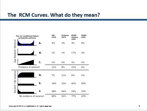See “The RCM Curves (Slides 7-18)” In this set of slides we learned that real world data has immense value. Understanding failure behavior depends on having acquired the ages of failure modes at failure and suspension.

Conditional probability of failure

Slide 2 Conditional failure probability confers power.

The most powerful information sought by all maintenance engineers and managers boils down to the conditional failure probability. It is the probability of an item failing in an upcoming period of interest given that it is currently in operation. If you knew that the conditional probability of failure of a part or component were unusually high you could channel your manpower to intervene propitiously, thereby preempting the consequences of a failure in service while avoiding waste of resources and unnecessary downtime on items where failure is not imminent.

What is the conditional probability?

Slide 3 What is conditional probability?

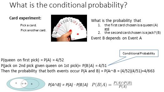
A little further down we’ll describe how to calculate the conditional probability of failure of an item. Right now we’ll discuss Conditional Probability itself and then we’ll define the Conditional Probability of Failure.

Let’s begin with a card experiment. A card is chosen at random from a standard deck of 52 playing cards. Without replacing it, a second card is chosen. What is the probability that the first card chosen is a queen and the second card chosen is a jack? The events are said to be dependent because the probability of the second depends on the first.

A. P(queen on first pick) = 4/52
B. P(jack on 2nd pick given queen on 1st pick) = 4/51, a higher probability than 4/52

Then the probability that both events occur P(queen first and then jack)= (4/52)(4/51)=4/663

The probability of choosing a jack on the second pick given that a queen was chosen on the first pick is called a conditional probability. The conditional probability of an event B in relationship to an event A is the probability that event B occurs given that event A has already occurred. The notation for conditional probability is P(B|A) ^[2].

When two events, A and B, are dependent, the probability of both occurring (denoted by “A∩B”) will, according to the card experiment, be the product of their probabilities, that is:

P(A∩B) = P(A) · P(B|A) , or $P(B|A)=\frac{P(A)\cap P(B)}{P(A)}$

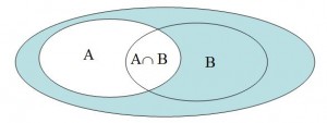
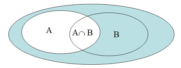
When two events are dependent (the probability of one depends on the other’s occurrence) their probability areas intersect in a Venne graphical representation.

What is the conditional probability of failure?

Slide 4 What is conditional probability of failure?

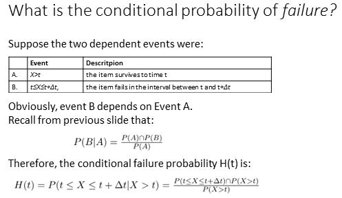
Suppose the two dependent events were:

X>t, an item survives to time t, X being the time of failure, and
t≤X≤t+Δt, the item fails in the interval between t and t+Δt given event 1.

As in the card experiment the probability of the second event depends on the first. Then the Conditional Probability of Failure is:

$H(t)=P(t\leq X\leq t+\Delta t | X>t)=\frac{P(t\leq X\leq t+\Delta t)\cap P(X>t)}{P(X>t)}$

It is the probability of failure in the interval between t and t+Δt (analogous to selecting a jack on the second pick) given that the item has survived to time t (analogous to selecting a queen on the first pick).

Slide 5 below shows that the conditional failure probability is a special case of the conditional probability where the numerator reduces simply to P(t≤X≤t+Δt). So that:

$H(t)=P(t\leq X\leq t+\Delta t | X>t)=\frac{P(t\leq X\leq t+\Delta t)}{P(X>t)}$

The conditional failure probability is a special case of the conditional probability

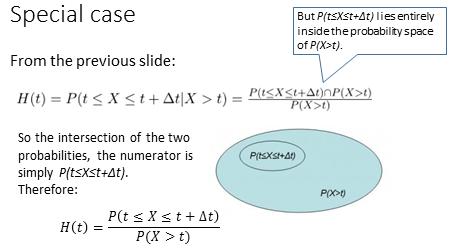
Slide 5 The conditional failure probability is a special case of conditional failure

X is the failure time. By definition the denominator is the survival or reliability function at time t, i.e. P(X>t) = R(t). The Conditional Probability of Failure is a special case of conditional probability wherein the numerator is the intersection of two event probabilities, the first being entirely contained within the probability space of the second, as depicted in the Venne diagram of Slide 5.

Conditional failure probability and reliability

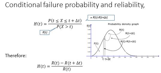
Therefore the numerator, which is the intersection of P(t≤X≤t+Δt) and P(X>t) reduces to simply P(t≤X≤t+Δt). Also, by expressing P(t≤X≤t+Δt) as the difference between the Cumulative Failure Probabilities calculated at t and t+Δt the numerator can be expressed as the change in Reliability over the interval Δt as:

P(t≤X≤t+Δt) = F(t+Δt) – F(t) = 1-R(t+Δt) – (1-R(t)) = R(t)-R(t+Δt)

where the Cumulative Failure Probability F(t) and the Reliability R(t) are complements, i.e. F(t) = 1-R(t), so that

$H(t)=\frac{R(t)-R(t+\Delta t)}{R(t)}$

What about the failure rate?

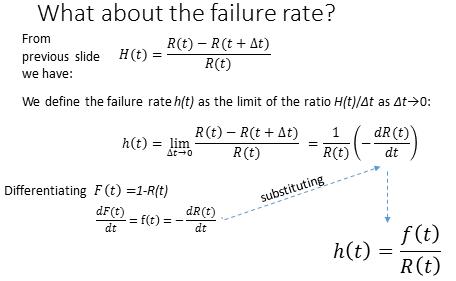
We define the failure rate^[1] h(t) as the limit of the ratio H(t)/Δt as Δt→0:

$h(t)=\lim_{\Delta t\rightarrow 0}\frac{R(t)-R(t+\Delta t)}{R(t)\Delta t}= \frac{1}{R(t)} \left ( -\frac{dR(t)}{dt} \right )$

Differentiating $F(t)=1-R(t)$ we have the density function f(t):

$f(t)=-dR(t)/dt$ :

Then

$h(t)=\frac{f(t)}{R(t)}$

Random failure. Is it really “random”?

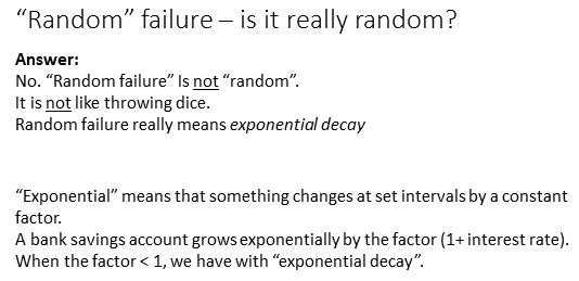
When something decays or grows “exponentially” it means that it changes regularly by a constant factor. An example of exponential growth is the principle in a compound interest bank account which increases at regular intervals by a constant factor^[1].

It’s not really “random” but rather “age independent”

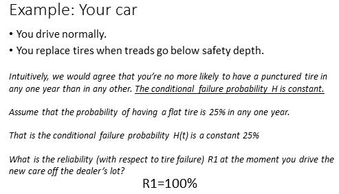Assume that you drive your car normally. You replace tires whenever the tread depth falls below the manufacturer’s safety recommendation. ^[2] Intuitively, we would agree that you’re no more likely to have a punctured tire in any one year than in any other.^[3]

In other words the conditional probability of failure (a flat tire) is constant or age independent. We call this failure pattern “random”.^[4] Assume that the conditional failure probability of a puncture in any year is a constant 25%. When you drive the car off the dealer’s lot for the first time, at that moment the Reliability R1 is 100%. What is the Reliability R2 at the beginning of the second year? In the article here we showed the Conditional Probability of Failure to be:

(1) $\begin{align*} H&=\frac{R_{1}-R_{2}}{R_{1}} \end{align*}$

Rearranging and substituting

(2) $\begin{align*} R_{2}&=R_{1}-H\times R_{1}\\ &=1-0.25\times 1\\ &=0.75 \end{align*}$

The reliability at the beginning of year 3 is:

(3) $\begin{align*} R_{3}&=R_{2}-H\times R_{2}\\ &=0.75-0.25\times 0.75\\ &=0.5625 \end{align*}$

Excel calculation and graph of Reliability and Conditional Failure Probability

Slide 10 Excel calculation and graph of Reliability (Survival) and Conditional Failure Probability

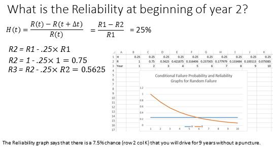
Repeating the calculation in an Excel spreadsheet for each subsequent year reveals the exponentially decaying Reliability curve of Slide 10.

Conclusion, so what?

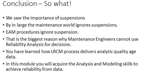
You have learned most of what you need to know in reliability theory. The real lesson is that the maintenance department, if it is going to leverage the principles of Reliability Analysis to develop optimal and verifiable decision rules, must capture the right information in the course of its day-to-day activities. Of prime importance is the distinction between failure mode instances that ended in failure and those that ended in suspension. In the upcoming sections,

“Weibull Exercises” and
“Optimal Preventive Renewal Exercises”
“The PF interval?”
“EXAKT Analysis and Model Building”
“Defeating CBM (reporting suspensions as failures)”

we will see how good data fuels practical decision making.

^[1]The factor is 1 plus the interest rate↩
^[2]This is an example of applying a Preventive Maintenance strategy in order to gain the desired constant, low conditional failure probability pattern.

If we allow the treads to wear beyond the safety depth then tire failure would become age related meaning that the conditional probability of failure would increase with age conforming to Nowlan and Heap’s pattern B.↩
^[3]Nevertheless the probability of surviving to an age t decreases with increasing age because, obviously, if you keep driving the car, eventually you will have a flat. This does not contradict the fact (although it seems paradoxical) that the probability of getting a flat in any one year, if you ask the question at the start of the year, remains constant.↩
^[4]The word “random” when used in the reliability sense differs from the often conjured image of throwing dice. In the latter situation it is impossible to predict the result of the next throw. To the Reliability Engineer, however, “random” means merely that the conditional failure probability in any interval is independent of the item’s age. Therefore, even when an item’s failure behavior is random, observed condition data can be used to predict its failure.↩

RA – Micro (day-to-day decision) analysis