Real meaning of the six RCM curves

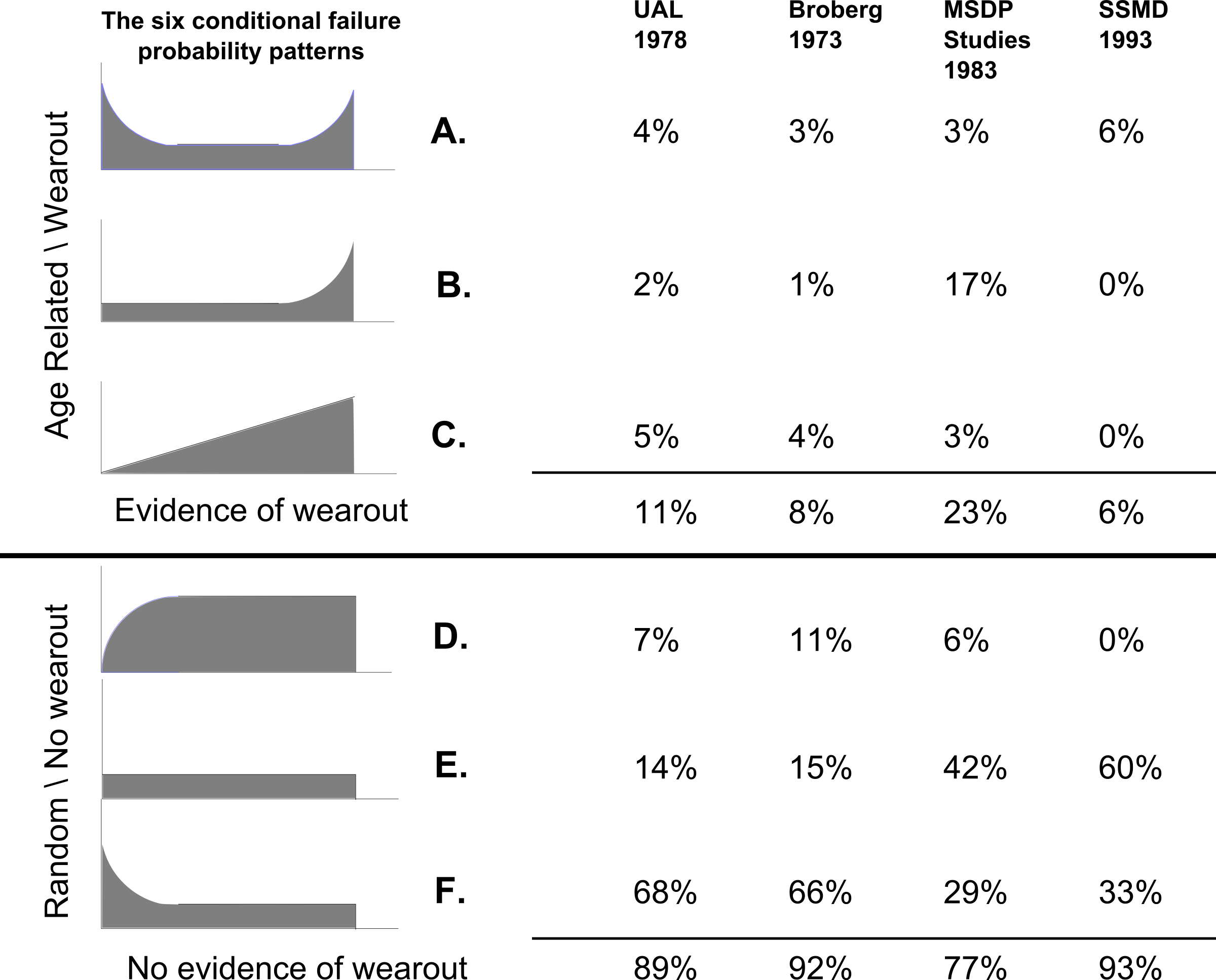
You may be wondering about the famous “RCM curves” shown below in Figure 1. They are the Age-Reliability behavior curves which graph the Conditional Probability of failure against age. A common question is the following.

“For the 139 items covered in the Nowlan & Heap (UAL) study, for example, do these curves represent the real failure behavior of the item? Or do they represent the “effective” net age-reliability relationship, given that most of these items were subjected to some form of age-based maintenance?”

Figure 1 The six RCM failure behavior curves^[1]

This is an excellent question. Many maintenance and reliability engineers are not completely sure of the answer nor of its underlying explanation.

Introduction

When one carries out so called “actuarial analysis” (more simply referred to as “reliability analysis”) to draw these curves, it is, indeed, to discover the true failure behavior of an item or failure mode^[2], regardless of the maintenance plan currently in force. How is this possible? Are we not basing our analysis on life data from equipment that has been maintained according to the maintenance strategy and schedule currently in force?

The explanation of this paradox lies in the actual observational data. At the time of maintenance (say, of the preventive renewal of a component) we will have made certain observations about the state of the maintained items. It is unlikely that we will have observed that all of the renewed items were on the verge of failure. Rather (unless the Preventive Maintenance (PM) plan is extremely conservative) some items will have failed prior to the moment of PM. That is, they will have failed in service. On the other hand, some of the renewed items will not have been in a failed state at the moment of PM. On the contrary, they would have been in excellent condition. Finally, indeed, some items will have well been “on their last legs” and just about to fail functionally. In those cases one might consider the PM as having been “well timed”.^[3]

An astute manager, made aware of the above observations, would undoubtedly ask “what is the optimal moment at which to conduct maintenance”. What PM schedule (termed a policy) will return the greatest benefit, i.e. give us the best overall availability, from a fleet perspective, over the long term? Our manager recognizes that being too conservative would be wasteful causing us to renew many perfectly good components. At the same time, he would not want to us be too liberal by selecting too long a maintenance interval. That would result in an excessive number of failures in service, increasing costs, and lowering overall reliability and availability.

Let us assume the true failure behavior were as shown below in the graph of Figure 2, which is Pattern B of the six failure behavior curves of Figure 1.

Figure 2 Conditional probability of failure curve for an item that ages – Failure Pattern B

Figure 2 plots the hazard rate or Conditional Probability of failure^[4] against the working age of an item. We would like to be able to claim (to our manager) that our maintenance plan has been optimized. That is to say, that we carry out maintenance at the working age represented by the useful life. The useful life would be the best time to do PM. Such a strategy would prevent most failures. Yet it would avoid renewal of very many items that are in perfect health. That optimum strategy would issue a PM action at a time of maximum benefit to the organization.

Obviously then, the graph of Figure 2 should represent the inherent designed-in age-reliability relationship of the item if we intend to use it to determine the useful life and, hence, the optimum age based maintenance policy. That brings us to the question, “How to draw this curve, given data from real world, maintained equipment?”

“Real world” implies that our calculations must take into account “suspended”^[5] data – data reflecting the actual preventive maintenance programs in place. The most popular and effective statistical method to discover the age reliability relationship is based on the Weibull model for life data. This is an empirical model discovered in the early 1950s by Walodi Weibull^[6], who presented the following probability distribution before an esteemed membership (who reacted with skepticism at first) of the then reliability engineering society.

Weibull Distribution – three of its forms

Figure 3 Three forms of the Weibull relationship

Probability density $f\left ( t\right )=\frac{\beta }{\eta }\left ( \frac{t}{\eta } \right )e^{-\left ( \frac{t}{\eta } \right )^\beta }$ (Eqn. 1)
Cumulative distribution $F\left ( t \right )=1-e^{-\left (\frac{t}{\eta } \right )^{\beta }}$ (Eqn. 2a), and
Reliability (aka Survival Probability) $R(t)=1-F(t)=e^{-\left ( \frac{t}{\eta } \right )^{\beta }}$ (Eqn. 2b)
Failure Rate $h\left ( t \right )=\frac{\beta }{\eta }\left (\frac{t}{\eta } \right )^{\beta-1 }$ (Eqn. 3)

Where:
β (beta) is the “shape” parameter,
η (eta) is the “scale” parameter, and
t is the working age of the item or failure mode being modeled.
F(t) is the Cumulative Distribution Function (CDF). It is the probability of failure in the period prior to age t.
R(t) the Reliability or Survival Function is the probability of the item surviving to age t. It is the complement of F(t)
h(t) is the Hazard or Failure Rate function and
f(t) is the Probability Density function.

One can convert algebraically from one to another of the above three forms of the Weibull relationship. For example, h(t)=f(t)/R(t).^[7]

Then we need only determine (estimate from historical data) values for the parameters β and η in order to plot the age reliability relationships of, for example, Figure 1. These graphs help us understand the age based failure behavior of items and failure modes of interest. Weibull developed a graphical method for estimating the values of the parameters β and η from a set of historical failure data. Today we do not need to use Weibull’s graphical estimation methods. Computerized numerical algorithms based on the Weibull model will estimate the values of β and η and plot the required graphs.

Example

For example, assume we have the following identical^[8] items, A, B, C, D, and E and the ages at which they failed.

Table 1:
Item	Failure age	Order^[9]
A	67 weeks	1
B	120 weeks	2
C	130 weeks	3
D	220 weeks	4
E	290 weeks	5

The Weibull method for finding the parameters β and η in Equation 2, $F\left ( t \right )=1-e^{-\left (\frac{t}{\eta } \right )^{\beta }}$ starts with a sample of life cycles whose values of F(t) at each of the failure ages 67, 120, 130, 220 and 290 weeks are known. That is, the Weibull method requires that we start by inserting reasonable values for the fraction of the population failing prior to the time t of each observation. That fraction will approximate the cumulative failure probability F(t)) at each of the five failure ages t.

Need for a better CDF estimate

We cannot simply assume that the value of the Cumulative Distribution Function F(t) is the percentage failed at time 120 weeks, i.e. 2/5, because that would imply that the cumulative failure probability (CDF) at 290 weeks, is 100%. Such a small sample size does not justify such a blanket, definitive statement.

To explain this more clearly, let’s extend the use of the simple fraction to the absurd, by considering a sample size of 1. We would not expect the age of this single failure to represent the age by which 100% of items in the sample’s underlying population would fail. It would certainly be more realistic to regard this single failure age as representing the age by which 50% of the underlying population would fail.

Therefore we need a better way of estimating the CDF, particularly for small samples of lifetimes, in order to apply it to the numerical Weibull solution for plotting the age-reliability relationship. The most popular approach to estimating the CDF from failure data is known as the median rank.^[10] A formula, known as “Benard’s probability estimator”, provides an estimate for median rank for small populations, and is given in Equation 4.

Benard’s probability estimator

$CDF \hspace{1}estimate=\frac{i-0.3}{N+0.4}$ (Eqn. 4)

Where:
i=the sequential order number of the failure; and
N=the size of the sample (number of life cycles)
CDF estimate=the Cumulative Distribution Function estimate, or Median Rank

Benard’s formula, applied to our hypothetical single failure, gives (1-0.3)/(1+0.4)=50%, which is intuitively reasonable.

We obtain, either from the median ranks table or from Benard’s approximation, the respective cumulative probabilities of failure (i.e. the CDFs). They are .13, .31, .5, .69, and .87. Of course, when we use reliability analysis software we do not, ourselves, need to look up the median ranks in tables or use Benard’s formula. A computer program applies median ranks automatically^[11] to each observation. The algorithm then applies a numerical (regression) technique known as the “Method of Least Squares Estimate” in order to estimate the values of β and η (depicted by their “hatted” symbols â and b̂ ) in the following equations:

Parameter estimation using regression

The following equations for estimating the Weibull parameters are explained at Weibull.com^[12] .

$\hat{a}=\frac{\displaystyle\sum\limits_{i=1}^r y_{i}}{r}-\hat{b}\frac{\displaystyle\sum\limits_{i=1}^r x_{i}}{r}$ (Eqn. 5) $\hat{b}=\frac{\displaystyle\sum\limits_{i=1}^{r}x_{i}y_{i}-\frac{\displaystyle\sum\limits_{i=1}^{r}x_{i}\displaystyle\sum\limits_{i=1}^{r}y_{i}}{r}}{\displaystyle\sum\limits_{i=1}^{r}x_{i}^{2}-\frac{\left(\displaystyle\sum\limits_{i=1}^{r}x_{i} \right)^{2}}{r}}{}$ (Eqn. 6)

$x_{i}=ln\left[T_{i} \right]$ and $y_{i}=ln\left[-ln\left[1-F(T_{i}) \right] \right]$ (Eqns. 7)

Where:
^ denotes that the value is an estimate.
Each F(T_i) is obtained from the Median Ranks or Benard’s Formula.
N=number of observations.
r(≤N)=the number of failures.
i is the sequential order number of each failure when all failures are listed in ascending order of failure age.

Once the computer algorithm has estimated a and b from Eqns. 5, 6, and 7, estimates for β and η can be found easily from â = -βln[η] and b̂ = β. Now any of the curves of equations 1, 2, or 3 may be plotted and examined to understand the item’s age based failure behavior.^[13]

Suspensions

Order

Now that we have discussed, in general terms, the Weibull method for plotting the age-reliability relationship (using historical failure data), we turn our attention to the problem of “suspensions”, which is the main subject of this article.^[14] Let’s begin with the sample of lifetimes in Table 2.:

Table 2
Item	Failure age	Order
A	84 weeks	1
B	91 weeks	2
C	122 weeks	3
D	274 weeks	4

The items are arranged in sequence according to their survival ages. Let N be the total number of observations, in this case, 4, and let “i” be the order (either 1, 2, 3, or 4) of a given failure observation. We can easily apply Benard’s formula to estimate the CDF at each of the four observations. Then we may proceed according to the methods discussed earlier, to determine the Weibull parameters and thus the age-reliability relationship.

Order with suspensions

But what if item B, for example, did not fail, but was renewed preventively, as directed, say, by the PM system? In such a case what would be the order “i” (of failure of items C and D) to be applied in Benard’s formula? We no longer know the orders of failure of items C and D because we do not know exactly when (beyond 91 weeks) item B would have failed (had it not been preemptively renewed).

Table 3
Item	Failure (F#) or Suspension (S#)	Failure or suspension age	Order
A	F1	84 weeks	1
B	S1	91 weeks
C	F2	122 weeks	?
D	F3	274 weeks	?

The table shows that the first failure was at 84 weeks. Then at 91 weeks an item was taken out of service for reasons other than failure. (that is, its life cycle was “suspended”). Two more failures occurred at 122 and 274 weeks. But the actual order of the failures of C, and D are unknown since they would depend on when B would have failed. Therefore their orders are indicated by “?”.

Using average orders

Suspended data is handled by assigning an average order number to each failure. The “average” is calculated by considering all the possible sequences as follows:

Had the suspended part been allowed to fail there are three possible scenarios (depending on when Item B might have failed had it not been suspended). In each of these scenarios the hypothetical failure of Item B is denoted by “S1 ->F” in Table 4.

Table 4
Possible Scenarios	i=1	i=2	i=3	i=4
Possibility 1	F1	S1-> F	F2	F3
Possibility 2	F1	F2	S1->F	F3
Possibility 3	F1	F2	F3	S1->F

Where:
F1 represents the first failed unit, Item A
F2 represents the second failed unit, Item C
F3 represents the third failed unit, Item D, and
S1 represents the first (and only) suspended unit, Item B, in this sample.

The first observed failure (F1) will always be in the first position and have order i=1. However, for the second failure (F2) there are two out of three scenarios in which it can be in position 2 (order number of i=2), and one way that it can be in position 3 (order number of i=3). Thus the average order for the second failure is:

$\frac{3 \times1+2 \times 2}{3}=2.33$

For the third failure there are two ways it can be in position 4 (order number of i=4) and one way it can be in position 3 (order number of i = 3).

$\frac{4 \times 2+3 \times 1}{3}=3.67$

We will use these average position values to calculate the median rank from Benard’s formula” (Equation 4), as in column 5 of Table 5, for use within Equation 7.

New increment

Table 5
Item	Failure or Suspension	Failure or suspension age	Order, i	Median rank
A	F	84 weeks	1	0.16
B	S	91 weeks	?
C	F	122 weeks	2.33	0.46
D	F	274 weeks	3.67	0.77

Obviously, finding all the sequences for a mixture of several suspensions and failures and then calculating the average order numbers is a time-consuming process. Fortunately a formula is available for calculating the order numbers. The formula produces what is termed a “new increment”. The new Increment I is given by:

$I=\frac{\left(n+1 \right)-\left(previous \;order \; number \right)}{1+number \;of\; items\; following\; the\; suspended\; set}$

Where
n=the total number of items in the sample;
I=the increment

So for failures at 122 weeks and 274 weeks the Increment will be:

$I=\frac{\left(4+1 \right)-\left(1 \right)}{1+2}=1.33$

The Increment will remain 1.33 until the next suspension, where it will be recalculated and used for the subsequent failures. This process is repeated for each set of failures following each set of suspensions. The order number of each failure is obtained by adding the “increment” of that failure to the order number of the previous failure. For example referring to Table 5, acknowledge that the Order of Item C (2.33) is indeed 1+1.33, and the Order of Item D (3.67) is indeed approximately 2.33+1.33.

Now that we have the adjusted orders of the failures, we can provide the F(t)’s^[15] required by Eqn. 7 for estimating the Weibull parameters using Regression.

Software

Figure 4 Analysis selection in SimuMatic

Although the foregoing seems rather complicated, the availability of powerful reliability software packages renders the job quite easy. For example, Reliasoft’s tool, SimuMatic, requires the user merely to enter or import the data and select the desired calculation method from the dialog (see Figure 4 ).

The Figure implies that there are several alternative calculation methods that can be used to estimate the age-reliability relationship. We have briefly described one of them, the Method of Least Squares Estimation with median ranking. Another popular method is known as Maximum Likelihood Estimation (MLE)^[16]. This article has attempted to provide the reader with some insight into the famous six RCM failure patterns (shown in the figure in the Introduction to this section), and, into the question, “How to know the true age-reliability relationship, from real world samples containing suspended lifetimes?”. The next part discusses the combining of the age-reliability relationship with business factors in order to establish an optimal preventive maintenance interval.

Optimizing TBM – cost model

Density function

Having understood the foregoing method for plotting the age reliability relationship, a practical question comes to mind. We may ask, quite legitimately, how knowledge of the age-reliability relationship can assist in optimizing the maintenance decision process? The following addresses this question.

Two useful ways to express the Weibull age-reliability relationship are as a:

Hazard function ^[17]
- The famous six RCM failure patterns (A-F) of Figure 1 represent the hazard function. Or as a
Probability density function,
- This form has some revealing visual characteristics as indicated in Figure 5:

Figure 5 Probability Density Graph

Conversion between the hazard and density functions is accomplished through the relationship h(t)=f(t)/R(t).

While the the density function, f(t), itself has no obvious ^[18] physical meaning, the area under the curve, F(t), is easily understood as the probability of failing before attaining a specified age t_P. Conversely, the grayed area, R(t), is the probability of surviving a mission of duration t_P. Since these are the only two possibilities the total area under the probability density curve is unity.

Expected unit cost

Now let us assume that t_p is the time at which, as a policy, time based renewal, is carried out. The obvious question then is, “what should t_p be so that it is optimal?”. By optimal, we mean that the organizational objective, say lowest operational cost^[19], is achieved. Let’s answer the question.

Equations 8, 9, and 10 below articulate (and resolve) the problem.

$c_{t}=C_{R}R\left(t_{p} \right)+C_{F}\left(1-R\left(t_{p} \right) \right)$ (Eqn. 8 )

$t_{t}=t_{p}R\left(t_{p} \right)+t_{F}\left(1-R\left(t_{p} \right) \right)$ (Eqn. 9 )

$\frac{C_{t}}{t_{t}}=\frac{C_{R}R\left(t_{p} \right)+C_{F}\left(1-R\left(t_{p} \right) \right)}{t_{p}R\left(t_{p} \right)+\int_{0}^{t_{p}}tf\left(t \right)dt}$ (Eqn. 10)^[20]

Where:
c_t is the expected (average) cost of maintenance due to both failure and preventive action.
t_t is the expected (average) age at which maintenance (either preventive or as a result of failure) takes place.
t_p is the age at which planned maintenance is to be performed. The objective of the analysis is to optimize the setting of t_p.
t_F is the expected or average time at which failure occurs.
C_R is the cost of a preventive action.
C_F is the cost of a corrective action which is greater than the cost of the preventive action.
C_t/t_t in Eqn 10 is the long run cost of maintenance (failure and preventive).

Equation 8 can be read as follows:

The expected operational cost, for the average life cycle c_t is equal to the cost of a preventive repair c_R multiplied by the probability that the item will survive until t_p, plus the cost of a failure induced repair c_F multiplied by the probability that the item will not survive until t_p.

A similar statement can be made for the expected time of actual maintenance, t_t, yielding Eqn. 9.

The maintenance manager is often interested in minimizing the overall expected cost (per unit of yielded product) of maintaining and repairing an item. This is expressed as a ratio, c_t/t_t in Eqn. 10. Equation 10 expresses the maintenance cost of an item relative to a “unit” of its usage. Equation 10 can be “solved” numerically for the value of t_p which minimizes the cost of maintenance in the long term. The software finds the t_p which minimizes^[21] the long run per unit of working age maintenance cost C_t/t_t.

Including condition monitoring data in the analysis

From a practical perspective the preceding analysis based solely on an item’s age severely limits the maintenance engineer. His day-to-day challenge is in deciding whether to intervene in an equipment’s current operation with a specific preventive action. Would doing so increase or diminish profitability? From the CMMS records the maintenance organization should know the item’s age and the age of its components.^[22] In addition to this age data, as a result of monitoring technology, the reliability engineer possesses additional information that can reveal the item’s condition. The question then is “How can the engineer extend the above described Weibull age based analysis to include relevant operational and condition information?

The extended analysis in EXAKT^[23] uses a Proportional Hazard Model (PHM) with time-dependent condition variables and a Weibull baseline hazard. The extended hazard function is:

$h\left ( t,\boldsymbol{Z}(t);\beta ,\eta ,\boldsymbol{\gamma} \right )=\frac{\beta }{\eta }\left ( \frac{t}{\eta } \right )^{^{\beta -1}}e^{\sum_{i-1}^{m}\gamma _{i}Z_{i}(t)}$ (eq. 11)

where β>0 is the shape parameter, η>0 is the scale parameter, and γ =( γ₁,γ₂,… γ_m,) is the coefficient vector for the condition monitoring variable vector Z(t)^[24]. In the extended analysis the parameters β, η, and γ, will need to be estimated in a numerical method. The resulting models contribute to the decision making capability of RCM and become part of the RCM knowledge base.

Conclusion

This article described the reasoning behind the six failure patterns that Nowlan and Heap revealed to the maintenance world in their pivotal work. Their report, entitled “Reliability Centered Maintenance”, was submitted on December 29, 1978 to the United States Secretary of Defense.^[25] The importance of RCM should not be underestimated. Its value extends beyond the discovery of the 6 failure rate patterns of Figure 1. Nowlan and Heap proved that effective maintenance can be achieved only when the maintenance department addresses all failure modes to an extent commensurate with their probability of occurrence and their consequences. An initial RCM analysis is carried out by experienced persons based on their best understanding or recollection of an item’s failures. Nowlan and Heap pointed out, however, that RCM analysis, even when conducted by knowledgeable persons, will be imperfect and tend to be overly conservative. RCM knowledge must be revisited and refined. Living RCM (LRCM)^[26] updates RCM analysis through a systematized assessment of maintenance related data. The LRCM process ensures that Reliability Analysis (RA) particularly when applied to the optimization of Condition Based Maintenance (CBM), will benefit from good information and data handling methods. Technicians, engineers, and managers, using LRCM procedures will, in a continuing process improve the RCM knowledge base, refine maintenance strategy and increase maintenance performance.

^[1]Reliability-Centered Maintenance (RCM) Handbook, United States Navy, http://www.everyspec.com/USN/NAVSEA/download.php?spec=S9081-AB-GIB-010_R1.030030.pdf ↩
^[2]A failure mode is the event that causes the failure. It can be defined as a particular part, component, or assembly that fails. Optionally the failure mode can include an action implying a physical change of state (e.g. fell off, jammed, etc). The expression of the failure mode may also terminate with a “due to” (e.g. fatigue, contamination, etc) clause. The level of causality at which to describe a failure mode will depend on the consequences of failure. Graver consequences will merit analysis at greater causal depth and the exploration of a larger number of (less likely) failure modes. It is an important RCM concept that the causality depth at which a failure mode is defined will not be homogeneous throughout the RCM analysis of a given asset. Some Failure Modes will require more depth and others less depth. Also see https://www.livingreliability.com/en/posts/how-much-detail/.↩
^[3]We refer to those imminent failures discovered as a result of inspection or other activities by the RCM nomenclature “potential failures”. Although the inspection has avoided the direst consequence of the failure, we still count potential failures as actual failures when calculating reliability performance indicators such as mean time to failure (MTTF).↩
^[4]The conditional probability of failure is the probability of failure in an upcoming relatively short age interval when the question is asked at the current moment. It is the most important reliability value for daily decision making. The difference between the Conditional Probability of Failure and the Hazard Rate is discussed here (https://www.livingreliability.com/en/posts/time-to-failure/).↩
^[5]When an item is renewed for any reason other than failure (or potential failure), its life is said to have been “suspended”. See section “Suspensions” below↩
^[6]Weibull, W. (1951) A statistical distribution function of wide applicability. J. Appl. Mech.-Trans. ASME 18(3), 293-297↩
^[7]For more information on the Weibull relationship see Reliasoft Wiki: The Weibull Distribution Chapter 8 http://reliawiki.com/index.php/The_Weibull_Distribution ↩
^[8]A legitimate objection raises the possibility that items A-E may be identical but may operate under varying conditions or duty cycles (harsher or less harsh). The analyst must take this into account by selecting an age measurement other than calendar time that normalizes usage. For example: “number of landings”, “number of rounds”, “litres of fuel consumed”, etc. Should variables other than working age be significant, for example, operating and condition monitoring data, then the Weibull age-reliability model must be extended to include CBM measurements. One such method is EXAKT.↩
^[9]The “order” is the sequence according to item age at failure.↩
^[10]For more information on the Median Rank tables and concepts see http://www.weibull.com/GPaper/ranks2_6.htm ↩
^[11]or uses another data fitting strategy such as Maximum Likelihood Estimation (MLE).↩
^[12]http://www.weibull.com/LifeDataWeb/estimation_of_the_weibull_parameter.htm. The only difference here being that Eqns. 5 and 6 account for the possibility of N-r life suspensions. Suspensions are a common occurrence in maintenance where parts or assemblies, not having failed, are nonetheless renewed preventively .↩
^[13]The numerical procedure will also yield statistical evidence that tells the reliability analyst whether and to what extent (with what confidence) the data indeed supports the Weibull model hypothesis.↩
^[14]Real world maintenance data will include not only failures but also preventive renewals (i.e. Suspensions) of items that did not fail. Not including suspensions would bias the analysis.↩
^[15]from the Median Rank tables or Benard’s formula↩
^[16]For more information on MLE see http://socserv.socsci.mcmaster.ca/jfox/Courses/SPIDA/mle-mini-lecture-notes.pdf ↩
^[17]The hazard function is also known as the “failure rate function” or, roughly, the “conditional probability of failure”. It is the probability of failure in the forthcoming relatively short interval of time, given that the item has survived to the start of that interval. An amusing story about the hazard function told by John Moubray can be found at https://www.livingreliability.com/en/posts/conditional-probability-of-failure-vs-hazard-rate/.↩
^[18]We might consider probability “density” as the “failure probability per unit of age”. Or, the rate of change of failure probability with age.↩
^[19]The objective could as well specify “highest availability” or a desired mix of high availability and high reliability and low cost.↩
^[20]The derivation of the denominator in Eqn 10 can be found in the post https://www.livingreliability.com/en/posts/expected-failure-time-for-an-item-whose-maintenance-policy-is-time-based/.↩
^[21]The objective could equally be specified as “highest availability” or a desired mix of availability and high “effective” reliability.↩
^[22]In reality most CMMS work order records do not accurately report Failure Modes. And few distinguish whether the ending Event Type was by Failure or by Suspension. This renders Reliability Analysis (RA) in maintenance impractical and usually impossible. Living RCM (LRCM) addresses this long standing problem.↩
^[23]A software driven analysis technique to include condition data with age data to automate condition based maintenance (CBM) decision making. See “https://www.livingreliability.com/en/posts/the-elusive-p-f-interval/“. ↩
^[24]For example the ppm of Iron and Lead in a sample of oil and the amplitude of vibration at a particular frequency could be elements in the vector of significant condition monitoring variables.↩
^[25]The work was performed by United Airlines under the sponsorship of the Office of Assistant Secretary of Defense (Manpower, Reserve Affairs and Logistics)↩
^[26]Reliability Analysis has consistently eluded the maintenance engineer due to the poor quality of work order historical (age) data. Our MESH LRCM product addresses two widely neglected yet vital issues:

1. How to attain high quality Age data consistently in the CMMS, and

2. How to ensure field experience is dynamically and accurately inserted into the RCM knowledge base and Reliability Analysis decision models. More information on the impact of low quality age data can be found at https://www.livingreliability.com/en/posts/defeating-cbm/↩

If you liked this article you may also enjoy

Failure declaration standards (48%)
EXAKT vs Weibull (32%)
The reliability data Catch 22 (32%)
Warranty for haul trucks (12%)
CBM Optimization (12%)
Templates for speeding up RCM (RANDOM - 8%)