A Condition Based Maintenance (CBM) policy is a procedure used by maintenance personnel to interpret a set of measured machine condition indicators and decide whether or not to renew a physical asset at the current moment.

Traditionally CBM data interpretive policies have been obvious. For example, if the glycol measurement in an engine’s lube oil is positive, the engine should be taken out of service and thoroughly inspected. Likewise for process machinery, if a temperature, pressure, or vibration reading exceeds a pre-defined limit, maintenance should be carried out before functional failure and secondary damage occurs.

However our ability to collect large amounts of condition data has continually outpaced our ability to define policies for its interpretation. Multiple measurement points in a process may be monitored and these health indicators may sometimes contradict one another. Upward or downward trends are frequently obscured by randomness in the data. In many instances no clear set of limits or rules have been developed to indicate whether or not a failure process is underway and how much time is available before the physical asset is no longer able to perform one of its functions.

The EXAKT CBM optimizing methodology was applied to a set of experimental condition data measurements in order to develop an optimal interpretation process or policy. An optimal policy is a procedure for data interpretation, which, if applied consistently in a CBM program, minimizes the cost of maintenance of a physical asset or maximizes its availability.

1. Introduction

Condition data from eleven gearboxes run to failure on the mechanical diagnostic test bed (MDTB) at Penn State University Applied Research Laboratory (ARL) was analyzed using the proportional hazards modeling (PHM) technique embedded in the EXAKT CBM optimizing program (see [1],[3]). Several statistical and replacement decision models were built based upon the observed condition data and ensuing failure events.

The MDTB makes a large number of condition indicators available for analysis, for example, the conventional vibration features such as acceleration amplitudes at various gear and bearing frequencies. In particular the Fault Growth Parameter (FGP) was calculated from the residual error signal obtained by a signal processing algorithm (see Miller) developed at ARL. We call it, henceforward, the ARL algorithm. In this algorithm, a family of Wavelets is constructed to decompose the gear motion error signal and extract the residual error signal for gear fault detection. In addition, we proposed a modified version of FGP called FGP1 by weighting each point in the residual error signal spectrum proportional to its deviation from a reference baseline. Besides FGP and FGP1, other useful indicators were extracted from the residual error signal. It was found that the revised version of FGP (FGP1) is superior to the FGP and other condition indicators for building the EXAKT model and making the replacement decision.

The eleven test runs were designated Test Run Numbers: 05, 06, 07, 08, 09, 10, 11, 12, 13, 14, and 15. All gearboxes were run in at 540 in-lbs torque for the first 96 hours of each test. Following the initial run-in period the output torque was increased as follows:

Test Runs 05, 06, 12, 13:	by 300% from 540 to 1620 in-lbs
Test Runs 07, 08, 09, 10, 11:	by 200% from 540 to 1080 in-lbs
Test Runs 14 and 15:	the load was alternated between 100% (540 in-lbs) and 300% (1620 in-lbs) at 30-minute intervals.

Vibration acceleration readings were taken at 8-hour intervals during the 96-hour run-in period and at 30-minute intervals during the high load ‘operational’ phase. Readings were of 10 seconds duration and sampled at a rate of 20 kHz. Accelerometers were located at various positions on the gearbox casing.

Test Runs 11, 13, and 15 ended in shaft failure. All other test runs ended with gear tooth failure. The gear ratio for Test Runs 05 to 11 was 1:1.533 and for 12, 13, 14, 15 was 1:3.333. We divide the test runs into two groups such that the gearboxes have the same gear geometry in each group: Group A is composed of Test Runs 5-11 and Group B consists of Test Runs 12-15. We found that the data from these two groups of physically different gearboxes have to be analyzed separately. “Gear tooth fracture” was the failure mode examined in this study. The three test runs where no gear tooth failure was observed were classified as suspensions.

In this paper, we analyze the data set described above and apply the EXAKT CBM optimizing methodology to develop optimal maintenance policies for the gearboxes. The paper is organized as follows. In Section 2, a signal processing technique is used to extract useful information from the raw vibration signals. Based on the extracted information, we obtain the event and inspection data that are essential to applying EXAKT. Data cleaning and pre-processing are also included in this section. In Section 3, EXAKT software is used to analyze the data, build PHMs for the gearboxes and develop optimal maintenance policies for them. Finally in Section 4, the results are summarized and some concluding remarks are given.

2. Data pre-processing and analysis

The original data provided by the ARL of Penn State University on a series of test runs of single reduction helical gearboxes contains vibration signatures captured by accelerometers mounted at different positions on the gearbox casing. As suggested by Miller [4], accelerometer A03, which is mounted in the axial direction, should be sensitive to the detection of helical gear tooth faults. Accordingly, data obtained from accelerometer A03 were used in our analysis. Since it is impossible to use directly the raw vibration data for the CBM analysis, a signal processing and data pre-processing step is required.

2.1 Vibration Signal Processing

In each test, data were collected until the MDTB was shutdown as a result of two accelerometers exceeding a predetermined limit of 150% of RMS. The targeted failure mode, tooth failure, however, may occur at any time prior to shutdown. To know the moment when the tooth failure really occurs, a signal processing technique is required. In the literature, there are many signal processing tools for vibration data (see, e.g., [2],[4],[5],[6],[7],[8]). Miller [4] proposed one such tool, the ARL algorithm. Miller used the Morlet wavelet filter (see, e.g., [9]) to decompose the motion error signal from the A03 accelerometer in order to make a diagnostic analysis based on the residual error signal plot. In addition, he proposed a fault growth parameter (FGP) to track the gear tooth health condition over time. The FGP is defined as the part (percentage of points) of the residual error signal which exceeds three standard deviations from the baseline residual taken when the run began.

The goal of signal processing in CBM is to filter out of the signal, as much operational and environmental data as possible, so that the magnitude of the remaining signal reflects the “ground truth” state of deterioration for the targeted failure mode. We modified the definition of FGP by assigning weights to the residual error signal points which exceed three standard deviations from the baseline residual. The weights were computed as proportional to the magnitude of their deviations. The modified version of FGP is called FGP1 in this paper. The signal processing technique described above enables us to prepare a table of inspection data related to the degradation process of the failure mode “tooth fractured” and a table of “event” data (installations, failures, suspensions, adjustments, etc). These tables are essential to applying the EXAKT procedure for creating statistical models supporting predictive maintenance decision making.

2.2 Event Data

To prepare the event data for applying the EXAKT CBM optimization technique, we are required to know when the gear was installed and when the gear tooth failure occurred. Also, other events, that would influence the measured variables or the failure mechanism, such as maintenance adjustments, operational changes, etc, should be included in the data. In this study, changes in torque loading as described in the introduction, were accounted for in the analysis process. The ARL algorithm was used as a method to detect the moment of tooth fracture providing the failure “event” data required for analysis. The event data for the gearboxes are presented in Figure 1.

In the events table “Ident” refers to Test Run number. “Event” refers to events: “B” designates the installation of the gearbox, “EF” designates the tooth failure event and “ES” designates the end of the test due to shaft failure (considered as a suspension with respect to the “gear tooth fractured” failure mode). “Date” is the calendar date and time when the event occurred. “WorkingAge” refers to the working age as a measure of service usage. Since, in each test, the gearbox operated under varying loads with torques ranging from 540 in-lbs up to 1620 in-lbs, it would be inappropriate to use simple calendar “running time” as a service usage measure, which would ignore the different working conditions under which the gearbox operates. As a reasonable approach we used the integral of the product of actual running time and instantaneous torque as the working age reflecting the accumulated stress on the gear teeth. The unit for working age, as defined, is in-lb-day.

2.3 Inspection Data

The signal processing technique is used to compile the table of inspection data related to the degradation associated with the targeted failure mode. Some tests ran for a period of time after failure occurred. Only inspections prior to detected tooth failure are included in the inspections table. For purposes of comparison some ‘conventional’ vibration features were also included in the inspections table. For example, the maximum amplitude of acceleration in a narrow frequency band around the gear mesh frequency and the sidebands, were tested as potential covariates in a proportional hazards model. The proportional hazards modeling analysis revealed, however, these are not significant indicators of gear tooth failure.

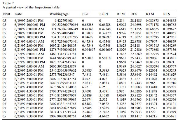
Inspection data are summarized as shown in Figure 2 which is a partial view of the entire Inspections table. “Ident”, “Date”, and “WorkingAge” have the same meaning as in the Events table. The other variables given in the Inspections table are:

FGP	fault growth parameter
FGP1	revised FGP
RFM	mean of the power spectrum of the residual error signal
RFS	standard deviation of the power spectrum of the residual error signal
RTM	mean of the residual error signal
RTS	standard deviation of the residual error signal

In addition to FGP and FGP1, RFM, RFS, RTM, and RTS were extracted from the residual error signal.

In the data set, there are several outliers that were reported by the ARL investigators as invalid data. Two significant outliers, one in Test Run 10 and the other in Test Run 14, were corrected by interpolating between the preceding and next values. The last three inspections in Test Run 11 have very high values. These abnormal readings may have been caused by contamination from other vibration sources as a result of the shaft failing. These three inspections were removed from the table prior to analysis.

2.4 Data Pre-processing

Before proceeding to the EXAKT modeling step, further investigation on the extracted features (called “covariates” in the analysis) was performed. First, FGP and FGP1 were compared over the test runs. FGP and FGP1 for a test run are plotted versus their timestamps on the same graph, as presented in Figure 3 and Figure 4.

From the graphs, we observe that FGP and FGP1 are almost identical for Test Runs 11, 13, 15, which ended as suspensions; and that FGP1 has larger values than FGP when the timestamp is close to the end of the test for all the test runs (Test Runs 5, 6, 7, 9, 12, 14) that ended in gear tooth failure. This is not very clear for Test Run 9. The relatively low values of FGP and FGP1 (and brief warning period) prior to failure in Test Run 9 might be explained by high variation in the reference baseline of the residual error signal. Using FGP alone, it is difficult or even impossible to distinguish between a failure history and a suspension history, (e.g., Test Run 14 and Test Run 15). Hence, we may expect that FGP1 is a better gear tooth failure indicator than FGP. It will be shown in the modeling phase that FGP1 is indeed a better indicator.

Next, correlations among the covariates were investigated for three cases: for data from Group A, for data from Group B and for the entire data set (Group A + Group B). Correlation analysis of the covariates is often useful to help in covariate selection in building a statistical (proportional-hazards) model. For each of the three cases, similar results were found, that is: FGP and FGP1 are highly correlated having a correlation coefficient of over 90%. Among the covariates RFM, RFS, RTM and RTS the correlation coefficients are over 90%. However, the correlation between any two covariates, one from the grouping of covariates FGP and FGP1, and the other from the grouping of covariates RFM, RFS, RTM and RPS, was relatively low (correlation coefficient less than 50%). It may be expected, then, that one representative from each grouping of covariates might be appropriate for inclusion as a covariate in the proportional hazards model.

3. Modeling and model analysis

Having prepared and validated the data as described, the next step is to build a proportional hazards model (PHM). The EXAKT software provides tools for selecting the covariates and building and analyzing the Weibull PHM (PHM with a Weibull baseline hazard).

The technique of PHM determines how the risk to failure, or hazard, depends on covariates. The influence of a covariate on the risk is expressed by the covariate parameters – covariate weights – which are the main outcome of the PHM analysis. The mathematical formula for the hazard at time t is:

The PHM is operating context specific. That is, if the physical asset’s operating context or mechanical configuration changes, then a different failure risk model (different covariate weightings) may apply. In the following subsection, we investigate whether the PHM depends on gearbox geometry. If so, we would be inclined to build two separate PHMs, one from each data set of Group A and Group B, rather than building a single PHM from the combined data of all test runs.

3.1 The Effect of Gearbox Geometry on the PHM

The physical configuration of the gearbox was changed in Test Runs 10-15. It is interesting to determine whether the PHM is unique to each gearbox geometry. An artificial covariate (also called a dummy variable) was created to denote the gearbox geometry. The value of the dummy variable is 0 if the test run is in Group A or 1 otherwise. We included the dummy variable and all other covariates to build a PHM. Then we removed (according to the PHM software procedure) each insignificant covariate, one by one, from the PHM until only the significant covariates (as determined by their p-values) remained. The dummy variable remained as a significant covariate in the model, which tells us that the risk model is different for different gear geometries. The PHM process is indicating to us that it is appropriate to build separate PHMs for Group A and Group B.

3.2 Analysis of Group A

Based on the correlation analysis discussed in Subsection 2.4, we may select either one covariate from the grouping of FGP, FGP1 or one covariate from the grouping of RFM, RFS, RTM, RTS, or one from each grouping (that is, two covariates in combination) to build a PHM. Since FGP1 outperforms FGP, we may only select FGP1 from the first grouping to build a PHM. PHMs for all three cases were examined. Other combinations were attempted but they did not yield better results than the aforementioned three cases.

In the analyses of Group A gearboxes, six different PHMs were investigated. The results for the six models with significant covariates are presented in Table 1. Also the model with both covariates FGP and FGP1 was analyzed and, as anticipated, FGP appeared not to be significant in that combination, although it is significant on its own. This means, simply, that FGP1 includes a greater amount of useful information than FGP.

The optimal replacement decision policy (see [1]) was calculated for each of the six PHMs. We used an estimate of the costs of failure and preventive replacement of $5000 and $1000 respectively. Alternatively, if maximum asset availability were the required optimization objective, one might apply a mean time to return to service (MTTR) of 1 week to 5 weeks respectively. To each policy there corresponds an optimal expected cost per unit of working age (given in the second column of Table 2). The column “Expected cost per in-lb-day” is the theoretical average cost (of both preventive and reactive maintenance) per unit working age determined at the minima of a graph of average cost versus risk. The “Average cost per in-lb-day applying the EXAKT decision policy” is the actual average cost that would have been expended had the optimal decision policy been in force during the sample.

From Table 2, we see that the decision policy based on model “RFS” yields the lowest expected cost, better than the second lowest yielded by the model FGP1. Which model should we choose for an optimal CBM data interpretation policy? In principle the best method would be determined by applying all these models in practice and to see which one gives the best results on average. That would be impractical. A “cost comparison” function in the software may be used to conveniently investigate the relative merits of alternative policies. The cost comparison in EXAKT generates the average cost per unit of working age calculated when the policy is applied retroactively to the data used in the analysis. The results of the cost comparison are summarized also in Table 2. The Cost Comparison function may be considered a final check of the statistical and decision model by reporting whether the decision model is useful, i.e. whether it improves current practice.

From the cost comparison it was found that models FGP1 and FGP1+RFM are similarly good (with average costs $0.231 and $0.233 respectively) and better than the other models. This could have been expected given the calculation methods and physical meanings of the variables. The difference between the theoretical and retroactively calculated costs (columns 2 and 3 of Table 2) may be explained by inaccuracies in the model parameter estimates due to small sample size. We may, nonetheless, consider models FGP1 and FGP1+RFM as good models, useful for the interpretation of CBM inspection data. In the model FGP1+RFM, the working age appeared non-significant ( ). We may prefer to use FGP1 as the final model because it is simpler, having only one variable.

Model FGP1 was applied to all seven histories from Group A. The decision graphs for these tests are presented in Figure 5. The optimal decision policy is applied by acting upon these graphs. If the point corresponding to the composite of the covariates lies in the green (lower) region of the graph, no maintenance action is recommended, in which case the expected remaining useful life (RUL), which is defined as the expected time to replacement due to either failure or preventive maintenance, is reported in the text box on the upper-right corner of the decision graph. If the point lies in the red (upper) region, the policy recommends immediate renewal. From Figure 5, we observe that the application of the model would have resulted in a recommendation to renew the gearboxes (which actually failed) prior to their failure. Furthermore, we observe that no recommendation would have been made to unnecessarily remove the unfailed gearboxes.

3.3 Analysis of Group B

Similar to the analysis of Group A, we analyzed Group B and obtained 5 tentative PHMs for Test Runs 12-15 as presented in Table 3. We observe that all models are independent of working age.

Again, the optimal expected costs per unit of working age and the results of the cost comparison for all models are summarized in Table 4.

From Table 4, we see that model FGP1 has the lowest expected cost per unit of working age. The model with the second lowest average maintenance cost is model RTS. The cost comparison, however, shows that model RTS is slightly better than model FGP1 (with average costs $0.306 and $0.311 respectively). Summarizing, we conclude that model FGP1 may be deployed as the final model. The decision model FGP1 is applied to Test Runs 12-15 and the decision graphs are presented in Figure 6. The FGP1 in Test Run 15 fluctuates slightly towards the later part of the test in response to the ramping up and down of load in the test. To remove the fluctuation of FGP1 and improve the model, we may use a smoothing function in EXAKT. The model was rebuilt based on the smoothed version of FGP1 and the decision graphs are presented in Figure 7. From Figure 7, we observe again that the application of the model would have resulted in a recommendation to renew the gearboxes (which actually failed) prior to their failure and no recommendation to unnecessarily remove the unfailed gearboxes.

5. Conclusion

Both the fault growth parameter (FGP) and its revised version (FGP1) provide a clear way to track the development of cracks or spalls in gear teeth. However the point at which a replacement action should be taken so as to respect some availability or cost criterion is not obvious. Using FGP or FGP1 in an optimization decision model results in setting a policy limit which responds to some stated economic objective for that physical asset, for example to minimize the total cost of failure and maintenance, to maximize physical asset availability, to attain a certain level of reliability, or to achieve a particular performance measure such as a target ratio of planned to breakdown maintenance. It has been shown that FGP1 is superior to FGP in fault detection and decision modeling. Maintenance managers can use the methods described here as a practical way to improve the return on investment in their existing CBM programs. The sample size of the data (number of histories, not number of inspections) analyzed in this paper is relatively low. Although larger sample sizes provide greater confidence, the MDTB test data was found to be adequate for demonstrating the usefulness of PHM and decision policy methodology described in this paper for predicting and preventing gearbox failures.

Acknowledgements We are most grateful to the Applied Research Laboratory at Penn State University and the Department of the Navy, Office of the Chief of Naval Research (ONR) for providing the data used to develop this work. We also thank Bob Luby at PricewaterhouseCoopers for his support. This work has been supported by the Natural Science and Engineering Research Council (NSERC) of Canada. The authors wish to thank NSERC for their financial support.

References

[1]. Jardine, A.K.S., Banjevic, D., Wiseman, M., Buck S. and Joseph T. (2001). “Optimizing a mine haul truck wheel motor’s condition monitoring program: use of proportional hazards modeling”, Journal of Quality in Maintenance Engineering, Vol. 7, No. 4, pp. 286-301.

[2]. Lin, J. and Qu, L. (2000). “Feature extraction based on Morlet wavelet and its application for mechanical fault diagnosis”, Journal of Sound and Vibration, Vol. 234, No. 1, pp.135-148.

[3]. Makis, V. and Jardine, A.K.S. (1992). “Optimal replacement in the proportional hazards model”, INFOR, Vol. 30, pp.172-183.

[4]. Miller, A.J. (1999). “A New Wavelet Basis for the Decomposition of Gear Motion Error Signals and Its Application to Gearbox Diagnostics”, M.Sc. Thesis, The Pennsylvania State University.

[5]. Miller, A.J. and Reichard, K. M. (1999). “A new wavelet basis for automated fault diagnostics of gear teeth,” Proceedings of Internoise 99, International Institute of Noise Control Engineering, Fort Lauderdale, FL.

[6]. Reichard, K. M. and Miller, A. J. (2000). “Wavelet-Based Filter Design for Gear Tooth Fault Diagnostics and Prognostics, Improving Productivity Through Applications of Condition Monitoring”, 54th Meeting of the Society for Machinery Failure Prevention Technology, Virginia Beach, VA, pp. 365-374.

[7]. Wang, W.J. and McFadden, P.D. (1995). “Decomposition of gear motion signals and its application to gearbox diagnostics”, Journal of Vibration and Acoustics, Vol. 117, pp. 363-369.

[8]. Wang, W.J. and McFadden, P.D. (1996). “Application of wavelets to gearbox vibration signals for fault detection”, Journal of Sound and Vibration, Vol. 192, No. 5, pp.927-939.

[9]. Young, R. (1993). Wavelet Theory and Its Applications, Kluwer Academic Publishers.

© 2015, Daming Lin. All rights reserved.