Expected failure time for an item whose maintenance policy is time-based

Let T_c be the time of a cycle, t_p the preventive maintenance time interval, and T the failure time.

The expected life cycle T_c will be the planned maintenance time t_p multiplied by the probability that planned maintenance does occur, plus the expected failure time (knowing that failure occurs before t_p) multiplied by the probability that failure occurs before t_p. This will be expressed mathematically by:

$E\left ( T_{c} \right )=t_{p}P\left ( T> t_{p} \right )+E\left ( T|T\leq t_{p} \right )P\left ( T\leq t_{p} \right )$ (Eqn. 1)

The term $E\left(T|T \leq t_{p} \right )$ in Equation 1, is the expected time to failure, given that failure occurs prior to scheduled maintenance, under a policy where scheduled maintenance is carried out at time t_p . We wish to show ^[1] that it can be expressed as

$E\left ( T|T\leq t_{p} \right )=\frac{\int_{0}^{t}tf\left ( t \right )dt}{1-R\left ( t_{p} \right )}$

First, we recognize that the conditional distribution function of $T|T\leq t_{p}$ is

(Eq 2)

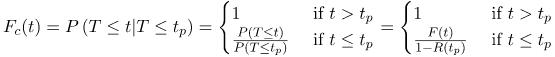
In the first part of Equation 2, we have simply defined the distribution function of (T≤t given that T≤t_p) as $F_{c}\left ( t \right )=P\left ( T\leq t|T\leq t_{p}\right )$ . We will call this conditional distribution function, “F_c(t)”. (Recall that this is the definition of a distribution function.)

Now, moving towards the right in Equation 2, the top condition “1, where t>t_p” is easy to understand. We know that failure will have occurred prior to t_p (with 100% certainty) because T≤t_pis our hypothesis in F_c(t).

The bottom case $\frac{P\left ( \left ( T\leq t \right ) \right )}{P\left ( T\leq t_{p} \right )}$ requires us to know that the conditional probability P(A|B) is $\inline \frac{P\left ( A\cap B \right )}{P\left ( B \right )}$ where A = T≤t and B = T≤t_p

But we know (in the bottom case) that the intersection of T≤t and T≤t_p is T≤t because the probability that T≤t is entirely within the probability space of T≤t_p (since t≤t_p is the bottom case). Therefore the intersection of T≤t and T≤t_p is actually T≤min(t,t_p)=T≤t.

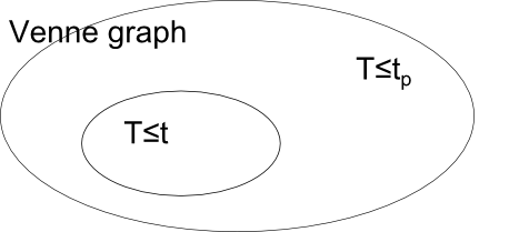
Venne Diagram

In the rightmost part of Equation 2 we apply the definition of F(t) to the numerator and denominator. And, of course, we know that F(t) = 1-R(t).

Then the conditional density function of $\inline T|T\leq t_{p}$ is

$\inline f_{c}(t)=\begin{cases} 0 & \text{ if } t> t_{p} \hspace 2 or \hspace 2 t < 0\\ \frac{f\left ( t \right )}{1-R\left ( t_{p} \right )} & \text{ if } 0\leq t\leq t_{p} \end{cases}$ (Eq. 3)

We have used, in Equation 3, the fact that the density function is the first derivative of the distribution function. Therefore,

$\inline E(T|T\leq t_{p})=\int_{0}^{\infty }tf_{c}\left ( t \right )dt=\int_{0}^{t_{p}}\frac{tf\left ( t \right )}{1-R\left ( t_{p} \right )}dt=\frac{\int_{0}^{t_{p}}tf\left ( t \right )}{1-R\left ( t_{p} \right )}$ (Eq 4)

Here, in Equation 4, we have invoked the definition of “Expectation” as the integral of the product of t and the density function.

^[1]in order to derive the denominator of Eq 10 of the post “Real meaning of the six RCM curves“↩

Expected failure time for an item whose maintenance policy is time-based

Search:

Categories

Forum topics

Other

Contact us: